Sports Prediction Algorithm Accuracy - How To Get It Right
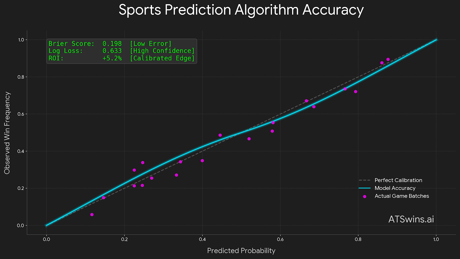
Table Of Contents
- Making Accuracy Mean Something in Sports Prediction
- What Accuracy Really Means in Sports Prediction
- Data and Feature Engineering That Actually Moves Accuracy
- Train Test Protocols That Avoid Illusions
- Calibration Expected Value and ROI
- Monitoring and Reporting in Production
- How to Build Calibrate and Report a Practical Sequence
- Tools and Templates That Save Time
- ATSwins Perspective Accuracy That Converts to Smarter Decisions
- Practical Accuracy FAQs for Sports Prediction Teams
- Worked Example From Raw Probabilities to a Bet Decision
- Segment by Segment Tracking That Reveals Where Accuracy Lives
- How to Talk About Accuracy With Leadership and Users
- How to Build Trust Accuracy Meets Transparency
- Quick Win Checklist to Raise Real Accuracy This Month
- Frequently Asked Questions
Making Accuracy Mean Something in Sports Prediction
Winning isn't just about calling the final score. It is about putting the right probabilities on each outcome. As a sports analyst who basically lives inside data models, I am going to show you how to measure prediction quality way beyond the raw hit rate. We are going to get into Brier scores, log loss, AUC, and exactly why calibration, expected value, and strict bankroll discipline are the only things that turn raw numbers into sustainable edges.
What Accuracy Really Means in Sports Prediction
Accuracy in sports prediction is definitely not just about asking how often we picked the winner. That is the amateur way to look at it. Hit rate, or your win percentage, is super easy to compute, but it is also incredibly easy to misread. You have to think about it this way. If your model calls every single NBA favorite correctly at a sixty five percent clip but never accounts for the price you are paying on the odds, you can literally lose money while feeling like you are accurate. In betting markets, you need calibrated probabilities and loss functions that reward both correctness and confidence. Since a lot of regular searches come up dry on this stuff, we have to lean on standard metrics literature like the Brier score and the theory of proper scoring rules.
Accuracy is not just a label you slap on a model. It is a distribution of probabilities tied to a decision rule and a bankroll. Win percentage measures classification, which is just picking a side, but it does not measure the quality of your probabilities. Proper scoring rules are there to reward well calibrated forecasts and penalize you when you get overconfident.
There are key metrics that actually reflect predictive quality. First, you have the Brier score. This is binary, like if Team A wins or loses. It is the mean squared error of predicted probability versus the actual outcome of zero or one. In this case, lower is always better. Then you have log loss or cross entropy. This penalizes confident wrong picks heavily. Lower is also better here. It is sensitive to extreme probabilities, which is often totally appropriate in betting contexts. You also have ROC AUC. This measures discrimination, or how well you rank winners versus losers. This is valuable with class imbalance, like when underdogs win less often, or when you want ranking quality. Higher is better for this one. Finally, you have calibration error, like Expected Calibration Error. This compares predicted probabilities to observed frequencies to see if your seventy percent predictions actually win about seventy percent of the time.
You have to understand why win percentage alone misleads you. Consider an NHL model that always picks the favorite. You might post fifty seven percent accuracy. If the average price is minus one hundred and sixty, which implies sixty one and a half percent, your edge is actually negative. You have good accuracy on paper, but bad expected value. Two models can show identical win percentages, but one could be better calibrated and produce much higher expected value after the odds are considered.
There is a simple way to think about these metrics. The Brier score rewards you for saying zero point seven one when your picks win seventy one percent of the time. Log loss punishes you for saying zero point nine nine and losing. ROC AUC judges whether your seventy percent predictions tend to be higher than your fifty five percent predictions for games that actually win, regardless of the threshold. Calibration tells you whether your stated probabilities match reality across different buckets.
If you want to compute and narrate accuracy beyond just win percentage, you need a step by step process. For each prediction and outcome, you calculate the Brier by taking the prediction minus the outcome and squaring it, then averaging that across games. For log loss, you use the standard formula involving logarithms of the prediction and the inverse prediction, averaging that across games too. For bucket calibration, you bin your predictions into groups like fifty to fifty five percent, fifty five to sixty percent, and so on. For each bin, you compute the mean predicted probability versus the actual hit rate and plot them on a reliability curve. For ROC AUC, you collect all probabilities and outcomes and compute the AUC to see the rank quality of your probabilities. You should also report confidence intervals via bootstrap by resampling games with replacement. You recompute Brier and log loss across a thousand bootstrap samples and show ninety five percent intervals so stakeholders see the variance, not just point estimates. You can keep a win percentage column, but you should label it clearly as thresholded classification, like probability greater than point five equals a pick. Never present it alone.
To compare them in your head, think about hit rate as a binary output that measures the accuracy of hard picks. It is good for simple reporting but ignores odds. Brier score is probabilistic and measures calibration and sharpness. It is great for day to day model health. Log loss is also probabilistic and penalizes overconfidence strongly. It is best for betting contexts with extreme probabilities. ROC AUC is a ranking metric that measures discrimination. It is good for imbalanced classes but ignores calibration entirely. ECE or calibration is probabilistic and measures the alignment of probability to frequency. It is crucial for aligning forecasts to action thresholds. For player props like yards or points, you will also use regression metrics like Mean Absolute Error and root MSE, or Continuous Ranked Probability Score when predicting full distributions.
Data and Feature Engineering That Actually Moves Accuracy
Messy inputs and leaky features will absolutely sink any model. ATSwins focuses on features that are stable before the decision cut off and that actually move the needle across the NFL, NBA, MLB, NHL, and NCAA.
You need clean, trustworthy data sources. You want historical box scores and play by play data to build consistent team and player features such as usage, true shooting, pace, EPA per play, wOBA, xG, and special teams strength. You also want market based baselines like closing lines, moneylines, spreads, totals, and derived implied probabilities. You have to use them carefully as a benchmark and as features only when allowed by your workflow. Injury reports and rest days are huge. You need official team reports, league feeds, and day of updates. For the NBA and NHL, back to backs and travel matter a lot. In the NFL, offensive line injuries and cornerbacks can swing win probability very quickly. Travel and altitude are also factors, specifically the distances between stadiums, days since the last game, altitude flags like in Denver, and circadian penalties for early starts. Weather for outdoor sports is critical, including wind, temperature, precipitation, and field surface. You must format weather features to match when forecasts lock before the game.
Closing lines need special care. If you are making a decision before the market finalizes, using the closing line as a feature introduces leakage. You have to treat the closing line as a baseline to beat, or use the last available pre deadline lines to avoid seeing the future. Recommended public data assets include the Sports Reference family sites for historical stats and rosters, official league injury and transaction feeds, and team PR feeds or beat reporters, provided you normalize the text into structured fields.
Feature engineering needs to map to outcomes. Practical team features include team strength ratings like Elo, recent form over rolling five to ten games, and schedule strength. You should look at pace and tempo adjustments, and possession estimates for totals. Set pieces and special teams like NHL power play rates or NFL special teams EPA are vital. Matchup interactions like frontcourt versus rim protection or pass rush versus quarterback time to throw are also key. Player centric features should include rolling usage and efficiency, on and off splits, and lines only replacements to see what the likely replacement is when a star sits. You need minutes projections and snap shares for the NBA and NFL. For MLB, you need handedness splits, park factors, and bullpen fatigue.
Market alignment and off market edges are important. Compare your fair probabilities to market implied ones adjusted for the book’s overround or vig. Store both as features to learn when your model tends to be right versus when market drift explains everything.
You absolutely must avoid leakage by freezing features at decision time. Timestamp every feature by an as of time. If your pick is made at twelve Eastern, you cannot use injury updates posted at twelve oh five. For lines and odds, log the latest pre deadline figure you actually saw. If you report closing line CLV, mark it as post outcome metadata, not a feature. When using rolling means, ensure they only use games that occurred strictly before the decision timestamp. Be careful with rankings and league averages that get updated later, and keep versioned snapshots.
Data hygiene stabilizes accuracy. Standardize identifiers for teams, players, and games, as well as time zones. Deduplicate events, especially with scraped feeds. Impute missing values with simple, documented rules, and flag imputed fields as separate binary features. Handle outliers by capping extreme values responsibly, but keep flags for extremes since they can carry signal, like fifty plus point NBA nights. Helpful tools for this include Pandas or Polars for feature pipelines, DuckDB for local analytics, Great Expectations or pandera for validation, and simple JSON schemas for injury feeds.
Train Test Protocols That Avoid Illusions
Random train test shuffles will totally overstate accuracy for time ordered sports data. You have to use time aware evaluation that respects causality.
You need chronological splits and walk forward evaluation. A basic chronological split might train on seasons up to 2022 and test on 2023. This is good for a single snapshot, but it underestimates uncertainty. Walk forward validation is better. You split the timeline into folds, train on the past, validate on the next segment, and roll forward repeatedly. This reveals stability across time. You have expanding windows versus rolling windows. Expanding means the training set grows with each fold, which is best when older data remains relevant. Rolling means the training window size is fixed and drops old data, which is best when the sport evolves quickly.
A practical, Python friendly way to do this is to use TimeSeriesSplit to keep order intact. For hyperparameter tuning, nest cross validation with an outer time based split for unbiased evaluation and an inner time based split for tuning.
Here is a step by step way to implement a solid backtest protocol. First, choose the forecast granularity, like game level win probability or spread cover, or player prop distribution. Second, create time folds. For example, train on 2019 to 2021 and validate on 2022, then train on 2019 to 2022 and test on 2023. Or do it monthly or weekly for the NBA and MLB. Third, define an untouched baseline using market implied probabilities or a simple Elo. Use it to benchmark Brier and log loss and to frame expected ROI after vig. Fourth, train inside each fold. Fit your model only on past data. Freeze feature transformations and scalers fitted on the training part of that fold. Fifth, evaluate by computing Brier, log loss, ROC AUC, and calibration by buckets. Report all with bootstrap confidence intervals. Sixth, make a single production pick file for each fold to avoid leakage. Include the timestamp, features as of that time, predicted probability, book odds at decision time, and the selected action.
Nested tuning without peeking is critical. In the inner loop, tune hyperparameters with time aware CV. In the outer loop, lock hyperparameters and score the model. Only outer loop results make it into your public accuracy numbers.
Confidence intervals matter because probabilistic metrics are noisy over small samples, especially in the NFL. Use block bootstrap by week or by day to capture serial correlation. For hit rate, use Wilson or Clopper Pearson intervals to avoid overly optimistic normal approximations when sample sizes are small.
You also need to backtest against robust baselines. Use a market baseline, which is the book implied probability adjusted for vig. Use simple rating systems like a vanilla Elo with home court and rest adjustments. Use naive heuristics like always picking the favorite or spread based thresholding. If your model does not beat the baseline on Brier or log loss across multiple folds with non overlapping confidence intervals, you likely have no edge. It is way better to know that early.
Calibration Expected Value and ROI
Raw probabilities are rarely perfect. Calibrating them improves decision quality and expected value.
You need to fit calibration and test it visually. Two standard calibration methods are Platt scaling, which is logistic regression on model outputs versus outcomes and works well for sigmoid shaped miscalibration, and Isotonic regression, which is a non parametric monotonic mapping that is flexible but needs more data to avoid overfitting. Use standard tools to fit calibration on a validation set, not the final test set. Plot reliability curves where the x axis is predicted probability and the y axis is observed win rate per bin. Compute ECE and report by segment.
The workflow involves splitting your predictions into train, validation, and test by time. Train the model on train and apply it to validation. Fit a calibrator like Platt or isotonic on validation predictions and outcomes. Lock the calibrator and apply it to test predictions. Evaluate Brier and log loss pre and post calibration, and pick the mapping that generalizes best.
You then convert probabilities to odds, edges, and actions. Fair odds from probability p in decimal format is one over p. In American odds, you approximate it. The edge against offered odds O in decimal is the expected value per unit stake, which is p times O minus one, minus one minus p. The edge percentage is just the EV. You bet if the EV is greater than your cost of risk threshold, including fees, limits, and estimated error. For example, if your model says p is zero point five five and the book offers plus one hundred ten or decimal two point one zero, the EV is zero point five five times one point one zero minus zero point forty five, which equals zero point one five five or fifteen and a half percent. That is attractive if your calibration is trustworthy.
Bankroll sizing with Kelly is the next step, but do it carefully. The full Kelly fraction for decimal odds O and probability p is p times O minus one divided by O minus one. Use Fractional Kelly, like a quarter or half Kelly, to reduce variance. Cap stake sizes by market liquidity and internal exposure limits. Even with a positive edge, variance can be brutal over short samples.
Tie your metrics to profit and loss without fooling yourself. After calibration, recompute EV and realized ROI. Show profit and loss versus a coin flip and versus a market baseline. Break results by odds segments like short favorites and long dogs because models often behave differently across price bands. Always display sample sizes and confidence intervals. Report drawdown statistics and max losing streaks.
Visuals that resonate with stakeholders include reliability plots of raw versus calibrated data, lift curves by odds bands showing model implied edge versus realized ROI, and time series of Brier and log loss to watch for drift.
Monitoring and Reporting in Production
Getting a backtest right is only half the job. Real world accuracy drifts with injuries, roster changes, weather, and market behavior. ATSwins treats production like a living system.
You have to detect drift early. Watch for data drift in inputs by monitoring summary stats and population stability index for key features like team pace or injury flags. Watch for prediction drift in outputs by tracking the distribution of predicted probabilities by market and time bucket. Watch for performance drift in outcomes by rolling Brier and log loss by week, ECE by bucket, and AUC for ranking stability.
Retraining cadence depends on the sport. For high volume sports like the NBA and MLB, consider weekly recalibration and a monthly model refresh. For lower volume or high variance sports like the NFL, recalibrate probabilities weekly, but retrain models on a multi week cadence to retain signal.
Guardrails on exposure are necessary. Implement a per market and per day cap to limit total units risked to avoid overexposure when signals cluster. Use stop loss and cool off rules so if realized ROI falls below a threshold over N bets, you reduce stake fraction or pause certain market segments. Check for odds movement. If the line moves heavily against your number before kickoff, reassess. This is especially important for props.
Post release testing involves A B and shadow deployments. Use a champion challenger model where you run the new model in shadow mode, logging its picks alongside the current model without sending bets. Use A B sharing to allocate a fraction of bets to the new model once shadow performance is confirmed under realistic latency and data conditions. Record end to end latency, missing data rates, and feature availability.
Explainability for stakeholders is key. Use global importance measures like SHAP or permutation importance to show which features consistently matter, like injury flags, rest, or travel. Look at stability over time to see if feature importance shifts season to season. Large shifts may signal data issues or structural changes in the sport. Use local explanations for occasional case studies on surprising picks, but keep these short and factual.
Dashboards should surface accuracy, not vanity. Report by sport, market, odds zone, and time. Show Brier score and log loss trends, calibration curves and ECE, and ROC AUC for ranking tasks. Show win percentage clearly as hard pick accuracy, secondary to probabilistic metrics. Make every chart clickable to surface bet level details like timestamp, features used, price at decision time, and the book. Given the lack of prior search findings, we spotlight broadly accepted methods backed by linked resources rather than niche or unvetted metrics.
Operational tips include versioning every model and calibrator used. Store the hash of the training data slice and feature spec. Keep a change log and weekly retrospective on what improved, what regressed, and any known incidents like an injury feed outage. Maintain a small canary set of games to sanity check outputs daily.
How to Build Calibrate and Report a Practical Sequence?
Here is a concise, repeatable sequence a small team can run in a week. First, do a data freeze. Lock the training cut off date and time and generate feature snapshots with as of timestamps. Second, build a baseline. Compute market implied probabilities, adjust for vig, and create a naive Elo or rating based baseline. Third, train the model. Choose a model family like logistic regression with interactions for transparency or gradient boosting for performance. Fit on the training window only. Fourth, do time aware validation. Use walk forward folds to estimate generalization and score Brier, log loss, and AUC per fold. Fifth, calibrate. Fit Platt or isotonic on validation and choose via log loss on a separate fold. Sixth, do the final test. Apply the locked calibrator to the untouched test fold and score metrics with bootstrap CIs. Seventh, define the decision rule. Convert probabilities to fair odds, define edge threshold and fractional Kelly stakes, and cap exposure. Eighth, backtest profit and loss. Compute expected and realized ROI by sport, market, odds band, and week, including drawdown stats. Ninth, report. Publish a one page report with Brier and log loss intervals, calibration plot, ROI by segment versus baseline, and pick volume with average implied edge. Tenth, go to production. Ship the model with feature time freezing, retry logic for data feeds, and monitoring dashboards.
Tools and Templates That Save Time
For modeling and evaluation, use logistic regression or gradient boosting. Simple linear models work when interpretability matters, while tree ensembles work when interactions help. Use reliability diagrams via standard library calibration curves. Use time aware CV with time series split functions. For data and engineering, use Polars or Pandas for pipelines, DuckDB for joins, and SQL for reproducibility. Use feature stores or simple parquet snapshots per day. For tracking and experiment management, use lightweight run tracking with CSV logs and hashes or experiment tools if you have them. Send daily monitoring reports via email or post them to an ops channel.
There are templates you can reuse. A model card one pager should include the objective, data window, features, training protocol, calibration, metrics, baselines, and known limitations. A backtest report per sport and market should include sample size, pick count, metrics, calibration plot, ROI, drawdowns, and operational notes. A weekly monitoring checklist should check if data feeds are healthy, if feature drift is within expected bands, if Brier and log loss are within control limits, if calibration slopes are stable, if exposure caps are respected, and if any model or calibrator changes were deployed.
ATSwins Perspective Accuracy That Converts to Smarter Decisions
ATSwins.ai provides data driven picks, player props, betting splits, and profit tracking across the NFL, NBA, MLB, NHL, and NCAA. Translating accuracy into real value means pushing beyond win percentage and tying every prediction back to calibrated probabilities and expected value.
ATSwins frames accuracy with a clear separation of metrics. Probability accuracy is measured by Brier and log loss reported by league and market. Discrimination is measured by AUC for ranking tasks. Calibration is measured by reliability curves and ECE so users know when a sixty percent tag really behaves like sixty percent. Market aware benchmarks are used against market implied probabilities instead of a coin flip. We label picks that are model favored but market opposed, with realistic expectations for variance. Player props realism involves reporting MAE and CRPS when we are using full predictive distributions, and calibration for over under outcomes. Prop edges can change rapidly with news, so features and calibrators are time frozen at pick release.
We turn probabilities into edges on the platform. Fair odds are printed alongside book odds where available, with implied edge and suggested unit size using fractional Kelly. Users can override aggression levels because bankrolls and risk tolerance vary. Exposure controls are built in with caps per sport and day, and per odds band limits to avoid stacking correlated risks like multiple overs on the same offense in the NFL. Variance disclosures ensure expected drawdowns and historical streak behavior are visible, so users understand the ride.
Accuracy reporting stays honest. Each pick carries a timestamp, data freshness notes, a pointer to the features used, the model version, and the calibrator version. It includes probability, fair odds, and edge, and post game realized outcome and closing price for context. Dashboards summarize rolling Brier and log loss and ECE by league and month, ROI versus market baseline with intervals and sample sizes, and odds band breakdowns to pinpoint where the model truly beats the market.
A realistic day to day flow keeps accuracy meaningful. In the morning, we do data checks, refresh injury and travel features, and freeze snapshots. Midday, we recalc probabilities, apply the calibrator, and publish picks that meet edge thresholds with exposure caps. Pre game, we monitor severe line moves. If the move is news driven and we missed it at decision time, we flag it but do not rewrite history. Post game, we update metrics, backfill realized outcomes, compute profit and loss versus baseline, and log any anomalies.
Practical Accuracy FAQs for Sports Prediction Teams
You might wonder if you should report win percentage at all. Yes, but always secondary to Brier and log loss and accompanied by ROI and sample size. Never present it as the only measure.
If your AUC is strong but calibration is poor, you can still extract value through calibration. A model that ranks well can be mapped to good probabilities with isotonic or Platt scaling.
Can you use closing lines as features? Only if you can access them at decision time. Otherwise, you are leaking future information. It is safer to use last available pre deadline lines and keep the true closing line as an evaluation benchmark.
If your NFL sample is small, how do you trust metrics? You have to aggregate across seasons with walk forward splits, use bootstrap intervals, and place more weight on calibration shape than on tiny differences in Brier or log loss.
Should you do per sport calibrators? Yes. Sports differ in scoring dynamics and market efficiency. Even within a sport, props and sides may need separate calibrators.
Worked Example From Raw Probabilities to a Bet Decision
Let's assume an NBA moneyline scenario. The model gives a raw probability that Team A wins of zero point five eight. The calibration mapping returns zero point five six. The book offers plus one hundred fifteen, or decimal two point one five. The fair odds from the calibrated probability are one divided by zero point five six, which is approximately one point seven nine.
Now we calculate the edge. The EV is equal to the probability times the decimal odds minus one, minus one minus the probability. That is zero point five six times one point one five minus zero point forty four. This equals zero point six four four minus zero point forty four, which is zero point two zero four. So, you have a twenty point four percent edge.
Next is the Kelly stake fraction. For decimal odds of two point one five, b equals the odds minus one, so one point fifteen. The fraction f star is equal to p times b minus one minus p, all over b. That comes out to roughly zero point one seven seven. If we apply a fractional Kelly of zero point three, the stake becomes five point three percent of the bankroll cap for this market.
Finally, we do exposure checks. If the daily market cap is ten units and this stake implies zero point five three units, we are within limits, so we place the bet. For reporting, we log the calibrated probability of zero point five six, fair odds of one point seven nine, offered odds of two point one five, EV of twenty point four percent, stake of zero point five three units, the model version, calibrator, and snapshot time. This example shows how accuracy connects to action, not just the binary label.
Segment by Segment Tracking That Reveals Where Accuracy Lives
Accuracy is rarely uniform. In odds bands, short favorites often have overstated confidence. Post calibration Brier and log loss should improve. If not, scale back stakes here. For long dogs, false edges arise from data sparsity. Use conservative thresholds and larger error bars.
In different sports and seasons, things change. The NBA has in season roster churn and scheduling density that raise drift, so retrain more often and calibrate weekly. MLB has a long season that allows robust estimates, but weather and park factors drive totals. The NFL has a small sample and high variance, so calibrate carefully and keep stakes conservative even when EV looks great.
Market types vary too. Totals often behave differently than sides, so use separate calibrators and features like pace estimates and weather. For player props, model distributions, not just means. For yardage, CRPS and MAE tell you more than binary over under hit rate.
How to Talk About Accuracy With Leadership and Users?
Stakeholders want clear metrics tied to money. They want to hear that log loss is down five percent versus last month, ROI is up two percent with the same pick volume, or drawdowns are cut in half due to exposure rules. They want evidence, not anecdotes, which means calibration curves, intervals, and consistent baselines. They want actionable next steps, like recalibrating props weekly, adding travel fatigue, or cutting stakes on long dogs until we collect more samples.
A simple accuracy brief template covers what improved this week, like Brier improving on NBA favorites or calibration slope getting closer to one. It covers what degraded, like NHL long dogs underperforming or realized ROI being negative despite model edge, leading to a decision to reduce stakes. It covers what we are shipping next, like injury report integration or new calibrators. And it covers risk flags, like weather feed instability for MLB totals requiring wider confidence bands.
How to Build Trust Accuracy Meets Transparency?
You have to disclose data freshness. State when features were last updated and what lags exist, like with injury feeds or weather updates. Put confidence intervals next to every key metric. No cherry picking allowed. Keep a public facing glossary. Define Brier score as measuring probabilistic error where lower is better. Define log loss as penalizing overconfidence heavily. Define calibration as the alignment of predicted probability with observed frequency. Define AUC as ranking quality, not probability quality. Reference accepted literature for your methods and standard tooling. These are battle tested and widely used.
Quick Win Checklist to Raise Real Accuracy This Month
If you want to raise your game right now, here is what you need to do. First, replace hard picks with probabilities everywhere. It is the only way to be real. Second, add calibration, starting with Platt, and compare your pre and post log loss. You will see the difference. Third, introduce a market adjusted baseline and stop comparing yourself to coin flips. The market is smarter than a coin. Fourth, shift to walk forward validation and add bootstrap intervals. Stop lying to yourself with random splits. Fifth, freeze features with as of timestamps to eliminate leakage. Do not peek at the future. Sixth, adopt fractional Kelly with exposure caps and publish the rules. Protect your bankroll. Seventh, build one dashboard section for calibration by odds band and keep it live. Finally, for props, predict full distributions when possible, then track CRPS and MAE.
Accuracy in sports prediction is the quality of your probabilities and your decisions under risk. It is tracked with proper scoring rules, defended by time aware evaluation, and expressed in calibrated EV and controlled exposure. That is how ATSwins treats accuracy, so bettors can make smarter, more informed calls day in and day out.
Conclusion
Accuracy is not just hit rate. It comes from calibrated probabilities, time aware validation, and bankroll discipline. The big takeaways are to use Brier or log loss, validate chronologically, and watch calibration and EV. Ready to act? Try ATSwins. ATSwins.ai is an AI powered sports prediction platform offering data driven picks, player props, betting splits, and profit tracking across NFL, NBA, MLB, NHL, and NCAA. Free and paid plans help bettors turn sound numbers into smarter decisions.
Frequently Asked Questions
What does sports prediction algorithm accuracy actually mean?
Sports prediction algorithm accuracy is not just win rate. It is how well your predicted probabilities match reality over time. If you say Team A has a sixty percent chance and, across many similar spots, they win about sixty percent, that is accurate. To judge this, use scoring rules that reward calibration and sharpness. Brier score measures squared error between your probabilities and outcomes, and lower is better. Log loss punishes overconfident wrong picks more than small misses, and lower is better here too. ROC AUC helps when you just need ranking quality, especially with class imbalance. In short, sports prediction algorithm accuracy is about honest probabilities and consistent value, not just how often you pick winners.
What metrics should I use to track sports prediction algorithm accuracy each week?
Keep it simple and steady. Use Brier score and log loss for probability accuracy. Use calibration curves to see if seventy percent predictions really win about seventy percent. Use ROC AUC if you care about ranking strength more than raw probabilities. Use expected value to connect probabilities to the market and your bankroll. If you work in Python, you can compute these with standard statistical libraries. Track them by league, market, and time. A small spreadsheet is fine and a weekly log is great, just don't overthink it.
Why can a high win rate still mean poor sports prediction algorithm accuracy?
Because win rate ignores odds. If you always pick big favorites at minus three hundred, you might hit seventy to eighty percent, yet still lose money when the rare losses wipe out gains. That means your sports prediction algorithm accuracy is weak in practice. Either your probabilities aren't calibrated, or you are betting prices without an edge. Good accuracy aligns your probability with fair odds, so your average bet has positive EV. Otherwise, a shiny record can hide negative ROI.
What are quick steps to improve sports prediction algorithm accuracy without overfitting?
Try this short, practical checklist. No magic, just things that work. Freeze features at decision time. Do not leak post game or post line move info into training. Validate chronologically with walk forward methods because random splits lie in sports data. Calibrate your model with Platt or isotonic and re check with a reliability curve. Start with strong baselines like market closing lines and simple Elo, then add signals like injury status, rest days, travel, and weather. Keep what helps, toss what doesn't. Monitor by segment, like league, market type, favorite versus underdog, or totals versus sides. Fix what drifts. Trim overconfident edges. If a bet shows huge EV, double check inputs because chances are it is data noise. Do these and your sports prediction algorithm accuracy will usually climb, slowly at first, then suddenly.
How does ATSwins.ai ensure strong sports prediction algorithm accuracy for users?
ATSwins.ai is an AI powered sports prediction platform offering data driven picks, player props, betting splits, and profit tracking across the NFL, NBA, MLB, NHL, and NCAA. Free and paid plans give bettors insights and guides to make smarter, more informed decisions. On top of that, we focus on sports prediction algorithm accuracy by calibrating probabilities and stress testing them against market movement. We track Brier score, log loss, and ROI by league and market so you see what is truly working. We turn probabilities into fair prices, EV, and suggested stake sizes with sensible exposure limits. We provide betting splits and profit tracking to spot drift early and adjust. You can learn more at ATSwins.ai, and yes, results are monitored over time, not just cherry picked days.
Related Posts
AI For Sports Prediction - Bet Smarter and Win More
AI Football Betting Tools - How They Make Winning Easier
Bet Like a Pro in 2025 with Sports AI Prediction Tools
Sources
The Game Changer: How AI Is Transforming The World Of Sports Gambling
AI and the Bookie: How Artificial Intelligence is Helping Transform Sports Betting
How to Use AI for Sports Betting
Keywords:
MLB AI predictions atswins
ai mlb predictions atswins
NBA AI predictions atswins
basketball ai prediction atswins
NFL ai prediction atswins
ai betting analysis