Ncaaf Late Season Regression Model - How To Price Late Form

Posted Dec. 11, 2025, 12:36 p.m. by Dave 1 min read

Late-season numbers can get wild enough to confuse even sharp bettors, especially when the narratives start taking over the moment November hits. As someone who builds AI models for sports analysis, I’ve had to learn how to pick apart what’s actually real and what’s just regression waiting to happen. The late season is where public perception tends to chase streaks, hot teams, cold teams, miracle quarterbacks, and overblown injury stories. But if you strip the noise and look at the right mix of priors, recent form, opponent strength, travel, injuries, and weather, you can actually pull out sustainable edges that last through the chaos. The entire point of what follows is to break down late-season regression and show how to blend different inputs into something actionable. You’ll get steps, tools, explanations, and enough examples to put this stuff to use instantly.

Table Of Contents

Tuning NCAAF Late-Season Regression for Smarter ATS Decisions
Data pipeline and feature engineering
Modeling strategy that balances simplicity and realism
Backtesting and deployment for Saturday slates
Practical build: from raw data to edges in five days
Handling injuries, fatigue, and travel with simple proxies
Mixing priors with recent form without overreacting
What not to do in November
Quality control: sanity checks before picks go live
Outputs that match ATSwins workflows
Example feature map for one November matchup
A short checklist to keep the build on track
References and tools (complementary, not competing)
Conclusion
Frequently Asked Questions (FAQs)

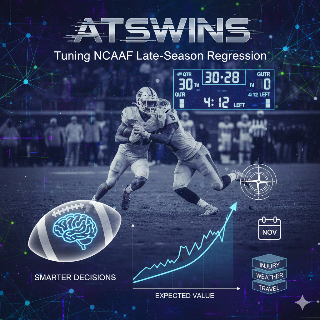
Tuning NCAAF Late-Season Regression for Smarter ATS Decisions

Late-season regression shows up everywhere in college football and it matters more in November than casual bettors realize. Regression to the mean is the idea that extreme performances end up drifting closer to normal over time. In college football, that can come from stuff like a quarterback having a massive efficiency spike for three straight weeks, a defense playing way above its normal havoc rate, or an offense posting explosive play numbers that are total outliers once you adjust for opponent strength. These things tend to normalize. The tricky part is figuring out which teams are genuinely improving versus which teams are hitting small-sample flukes that will fade fast.

There are two things people often mix up, especially in late October and November when the noise gets louder. The first is simple regression to the mean. If a team posts outlier stats against weak opponents or in weird weather games or in matchups where their strengths perfectly aligned with the opponent’s weaknesses, you should expect those numbers to flatten. The second is actual improvement or decline. Teams change late in the season because of injuries, scheme changes, depth issues, weather environments, or even switching quarterbacks. Those are real and can shift the true underlying team strength. If you don’t separate one from the other, almost every bet becomes guesswork.

For betting against the spread, this separation becomes crucial. Markets lean heavily on the last few games, especially when the public is drawn to recent trends. If you only chase recent form, you’ll end up paying inflated prices. But if you only lean on what happened in September, you’ll miss the stuff that actually matters now that roster health, weather, and fatigue have taken over. The sweet spot is blending season-long priors with recent opponent-adjusted form. Once you blend the two and shrink the recent window back toward something stable, you stop overreacting to the last week or two and you land on more grounded predictions.

A reality check worth keeping in mind is that you won’t find a perfect model that claims to solve NCAAF late-season regression because college football is too chaotic. The best you can do is build something structured that absorbs noise without drowning in it. Most of the time, sticking to domain fundamentals and good data is already enough.

Key late-season factors that deserve careful handling include small samples, opponent adjustments, injuries, continuity, fatigue, travel, and weather. Small samples are obvious. A three-game stretch doesn’t tell you much unless you look at who those games were against. Opponent adjustments help you avoid mistakes like thinking a team that blew out two weak pass defenses suddenly turned elite. Continuity is massive in November. Offensive line gaps, quarterback changes, cornerback injuries, linebacker depth, and general fatigue all start to matter more. Weather also becomes real. Wind, cold, and precipitation impact passing efficiency, pace, finishing drives, and even special teams. And travel adds another layer since certain conferences require cross-country games that hit harder late in the season.

If you’re building a model with ATSwins workflows in mind, all this becomes part of your output. The goal is to build stable predictions that reduce variance and produce consistent edges. You don’t need to find massive mismatches. You just need to find enough repeatable edges to outperform the close over time. Most of these edges come from correcting for market overreactions and understanding when a team’s recent stretch is fake heat rather than legitimate progression.

Data Pipeline and Feature Engineering

A good data pipeline for late-season modeling doesn’t need to be insanely complicated. The priority is making it clean, consistent, and timestamped correctly. Data integrity matters way more than fancy methods. Once you have something stable, you can use it every week without making massive adjustments.

Start by collecting schedules, box scores, play-by-play, and market lines for all FBS games. From that, compute team-game features like EPA per play, success rate, finishing drives, explosives, havoc, pace, and field position. These give you a basic structure to work with across phases of the game. After building the base features, adjust them for opponent strength using rolling opponent ratings. Then merge injury and continuity info with depth indicators, especially for quarterbacks, offensive lines, and defensive backs. From there add weather, travel distance, altitude, and rest days.

Create rolling windows, usually three to five games, and blend those with season-long priors using shrinkage. Define targets like ATS cover margin, spread error, or team total error. Timestamp everything so you don’t leak future information into past predictions. Split data by week to build blocked time-series validation. Keep every transformation and feature dictionary versioned so you can always reproduce your output.

When building targets, the primary one is ATS cover margin, which is actual margin minus closing spread. You can also define spread error or total error, but the core idea is always the same. You want the model to learn how teams perform relative to the market close because the close captures the most informed version of market activity.

The best features to use late in the season are opponent-adjusted offensive and defensive EPA, success rate, finishing drives, explosiveness, havoc, pressure rate, run-blocking signals, and efficiency splits across standard and passing downs. For game environment, include pace, field position, special teams proxies, weather inputs like wind and temperature, travel distance, and rest. For personnel and continuity, include returning starter indices, quarterback continuity streaks, offensive line injuries, and secondary availability. For market context, include opponent strength proxies from rating systems and the closing spread and total.

Opponent adjustment can be done in different ways, but two straightforward ones are weighted opponent indexing and ridge-stabilized fixed effects. Weighted opponent indexing subtracts the opponent’s defensive averages from your offensive performance and vice versa. Ridge-stabilized rating extraction uses simple regression to estimate offensive and defensive strength across teams. Either one gets the job done without unnecessary complexity.

Rolling windows need shrinkage so they don’t whipsaw you. Blended metrics mix recent performance with season-long averages. The weights depend on sample size and difficulty. For example, if you have five games against average opponents, you might weight recent form at around 0.4. If it’s only three games and the opponents were weak, maybe use 0.2. Shrinkage helps limit overreaction and keeps your output grounded.

Data hygiene is crucial. Always timestamp injuries and weather. Avoid final statuses when modeling openers. Normalize pace. Handle wind correctly. Drop duplicate or shifted games. Keep the pipeline clean so your modeling isn’t polluted by avoidable mistakes.

Modeling Strategy That Balances Simplicity and Realism

The modeling strategy should start simple and grow only when necessary. Basic regressions like OLS, ridge, and lasso often outperform more complex approaches when sample sizes are small. OLS gives you baseline interpretations. Ridge and lasso help handle multicollinearity and feature selection. Begin with features like opponent-adjusted EPA, pace, weather, travel, quarterback continuity, offensive line injuries, opponent strength, and market context.

From there you can build hierarchical Bayesian models that treat teams and weeks as random effects. This helps handle small-sample volatility and gives you natural uncertainty intervals. With Bayesian models, you can allow partial pooling across teams and weeks so extreme observations have less impact. Interactions can then be added in ways that reflect football reality. Examples include weather interacting with pass rate over expected, offensive line injuries interacting with pressure allowed, and tempo interacting with depth.

Make sure you penalize interactions so they don’t run wild. College football data has noise from blowouts, trick plays, garbage time, and weird weather, so you may want to use robust loss functions or trim extreme values. Garbage time can be its own feature so the model learns how late-game noise affects statistics.

For validation, never use random cross-validation splits. Use blocked time-series folds so the model predicts the future only from the past. Calibration matters too. Convert predictions into probabilities, then calibrate uncertainty bands based on historical residuals. Your goal is to produce predictions that give reliable cover probabilities and confidence intervals.

Backtesting and Deployment for Saturday Slates

A reliable model matters only when it’s deployed well. For weekly slates, simulate them with timestamp-safe historical data. Lock the available information as of Friday night or Saturday morning. For each week, generate edges relative to the closing line and organize them by size. Scorecard metrics should include edge distribution, hit rate by edge bin, net units after vig and realistic limits, and overall stability across the season.

Betting logistics matter. Assume you pay standard vig and can’t always catch the best price. Cap stakes per game and avoid stacking correlated plays. Use fractional Kelly for bet sizing so you don’t overextend yourself. For example, 25 to 50 percent Kelly is usually enough and you can scale it down in late-season volatility. Always manage correlated risk across conferences, totals, sides, and derivative markets.

Check weekly drift by comparing your predicted lines to the close. If you’re consistently off in weather games or games involving certain conferences, fix the model. Track injury lags where unexpected availability or snap counts broke the projection. Watch for signs of overfitting like coefficients flipping direction without football logic to support them.

Practical Build: From Raw Data to Edges in Five Days

If you want a fast mid-season build, you can knock it out in five days. Day one is data ingestion. Day two is feature building. Day three is creating targets and baseline models. Day four is building hierarchical models and interactions. Day five is backtesting and deployment. Once it’s built, you iterate each week to refine calibration and fix drift.

Handling Injuries, Fatigue, and Travel With Simple Proxies

Real-time injury data is messy in college football. You’ll need simple proxies. Quarterback continuity is one. Offensive line continuity is another. Defensive snap fatigue helps with late-season performance. Travel flags, rest days, and distance bands also help. These proxies are simple but surprisingly powerful because they capture stuff that’s hard to quantify perfectly.

Mixing Priors With Recent Form Without Overreacting

A consistent late-season mistake is ignoring early-season data. Keep it and reweight it. Start with season priors, add recent opponent-adjusted windows, and decay preseason experience. For quarterback changes, allow the model to shift the offense’s prior after around two games. This helps reflect real evolution without chasing short-term noise.

What Not to Do in November

Avoid chasing short-window extremes, double-counting injuries, using non-closing lines in labels, ignoring special teams, or dumping in too many correlated features. November is full of traps that can break models quickly if you’re not careful.

Quality Control: Sanity Checks Before Picks Go Live

Before pushing picks, check coefficient direction, residual clustering, and stability. Make sure changes in predictions week to week make sense. If predictions jump three points from last week without any major injury or weather change, something is wrong.

Outputs That Match ATSwins Workflows

Every model pick should include predicted cover margin, probability of covering, key drivers, confidence bands, and notes about correlation with other plays. ATSwins pushes clarity, transparency, and risk awareness, so your output should reflect that. Weekly drift monitoring and bankroll tracking are also essential.

Example Feature Map for a November Matchup

Take a typical late-season Big Ten game with cold weather and strong wind. You’d need opponent-adjusted rush EPA, line yards, defensive havoc, blended pace, weather flags, quarterback continuity, offensive line continuity, travel flags, and market context. The model will naturally shift toward slower games with more conservative offensive expectations.

A Short Checklist to Keep the Build on Track

Use closing lines for targets. Blend windows with priors. Adjust for opponent strength. Timestamp everything. Add football-relevant interactions. Validate with walk-forward splits. Calibrate uncertainty. Simulate slates. Control correlated risk. Track drift. Fix instability.

References and Tools

Reliable data includes official NCAA stats, historical play-by-play, and simple regression toolkits. Tools like hierarchical Bayesian packages help when you're ready for deeper modeling. The main goal is combining regression principles with opponent adjustment, injury awareness, weather effects, and bankroll discipline. That blend turns data into sustainable value, especially on a platform like ATSwins where everything is built to help bettors make smarter decisions built on actual math instead of hype.

Conclusion

This guide focused on pricing late-season NCAAF performance through regression, blending priors with rolling performance, adjusting for opponent strength, and accounting for injuries, travel, fatigue, and weather. The biggest takeaways are trusting mean reversion, using calibrated probabilities, validating on future weeks only, and tracking drift weekly. The late season is noisy but it’s also full of opportunities when you handle inputs correctly. When you combine all that with an AI-powered platform like ATSwins, you get consistent, grounded edges that build real value instead of relying on guesswork.

Frequently Asked Questions (FAQs)

What is an NCAAF late season regression model and how does it price late form?

A late-season regression model blends full-season opponent-adjusted metrics with the last few games to create a stable estimate of team strength. The idea is to mix long-term truth with short-term signals but shrink the short-term data so it doesn’t trick you. The final result is a fair number that you compare to the market to find edges.

Which data should I feed the model?

Use opponent-adjusted efficiency metrics like EPA per play, success rate, finishing drives, explosiveness, tempo, field position, special teams, and turnover luck. Add late-season signals like quarterback health, offensive line continuity, travel distance, rest, weather, and altitude. These stabilize predictions and add context.

How do I blend priors and recent games without overfitting?

Use shrinkage. A practical mix is giving around 70 to 80 percent weight to season-long metrics and 20 to 30 percent to recent games. Opponent strength affects the weights. Validate using walk-forward testing. If the model drifts, adjust the weights.

How do weather, travel, and injuries get added?

Treat them as inputs that interact with play style. Wind reduces passing efficiency more than rushing. Travel and rest affect pace. Offensive line injuries lower finishing drives and increase pressure rates. You can capture these with numeric and binary features like wind speed, precipitation, miles traveled, rest days, and starters out.

How does ATSwins use a late-season model?

ATSwins uses AI-powered data to generate picks, probabilities, and confidence bands. It blends season priors with recent form and produces outputs that help bettors make informed decisions without chasing noise.