

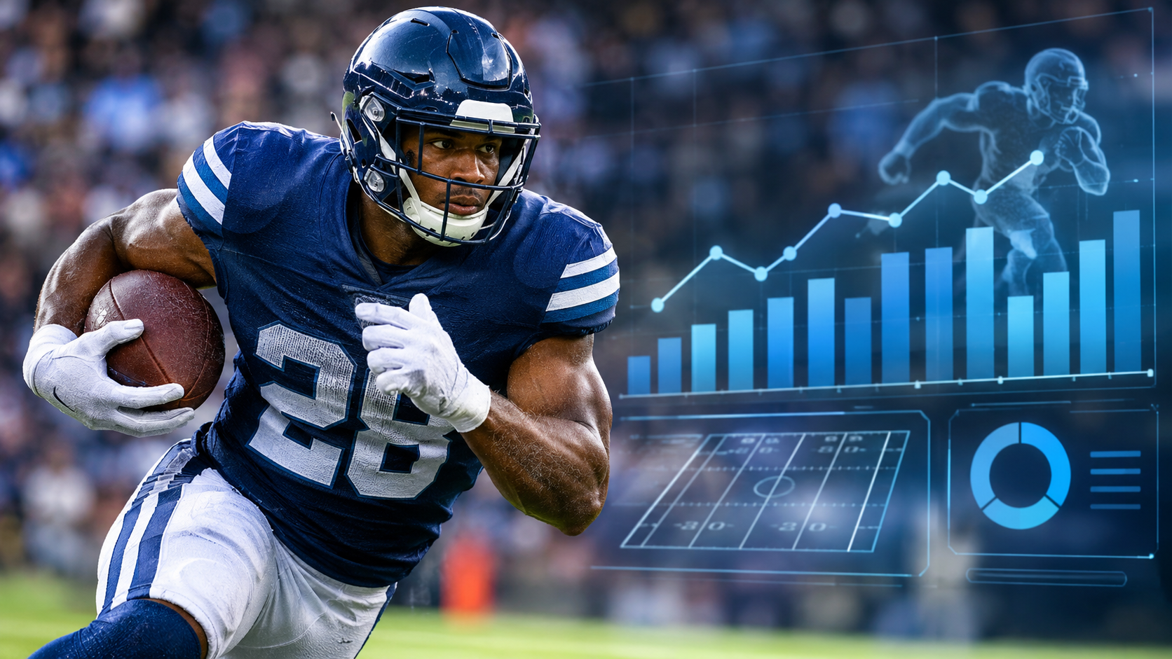
NFL running back rushing yards AI forecasts estimate how much ground a player is likely to gain in an upcoming game by combining workload projections, rushing efficiency, opponent tendencies, offensive conditions, and game-flow expectations. Instead of relying exclusively on season averages, statistical models evaluate the circumstances that could influence a player's next performance.
A useful forecast needs to answer two different questions: How many rushing yards should a running back be expected to produce, and how likely is that player to finish above or below a particular yardage threshold?
Those questions are related, but they are not interchangeable. A player projected for 78 rushing yards does not automatically have a strong probability of exceeding a 75-yard line. Workload uncertainty, matchup conditions, and the distribution of possible outcomes all matter.
Understanding those differences makes AI-based NFL player projections more useful for evaluating individual performance.
How AI Rushing Yards Forecasts Work
An NFL rushing projection begins with an estimate of opportunity.
A running back cannot accumulate rushing yards without receiving carries. That makes projected rushing attempts one of the most important components of any player forecast.
The model then estimates how efficiently those opportunities might translate into yardage. Historical yards per carry, opponent defensive performance, offensive-line conditions, rushing formations, and the player's role provide useful information.
A simplified projection framework looks like this:
Expected rushing yards = Expected rushing attempts × Expected yards per attempt
For example, a running back projected for 18 carries at 4.3 yards per attempt would have an estimated rushing total of 77.4 yards.
This calculation provides a starting point, not a complete forecast. A statistical model must account for the possibility that the player receives fewer carries, faces an unusually difficult defensive front, breaks a long run, or loses opportunities because of game circumstances.
Machine learning models can evaluate relationships across many historical observations, while simulation methods can generate thousands of possible game outcomes.
The objective is not to identify one inevitable result. It is to estimate a reasonable range of outcomes and assign probabilities to them.
The NFL has also demonstrated how advanced modeling can improve rushing analysis. Its Next Gen Stats Expected Rushing Yards framework evaluates player-tracking information, including the positions, speeds, and directions of blockers and defenders around the ball carrier. The resulting metrics distinguish actual rushing production from what the situation statistically suggested should have happened.
This is an important distinction: measuring what a runner was expected to gain on an individual carry is different from forecasting his total rushing yards for an upcoming game.
The second problem requires predicting both opportunity and performance.
The Data Behind Running Back Projections
Reliable NFL running back projections require several categories of information. No single statistic captures everything that determines rushing production.
Historical performance establishes a baseline, but the model also needs to understand whether the player's circumstances are likely to remain similar.
Recent production and season averages
Season rushing yards, carries, yards per attempt, and rushing yards per game provide an initial performance profile.
However, averages can conceal meaningful changes.
A running back might average 82 rushing yards across a season while receiving substantially more carries during the last three games. Another might have an impressive average because of one unusually long touchdown run.
A useful model separates ordinary rushing production from unusual performances and examines whether recent changes reflect a genuine shift in role or simply random variation.
Recent games should inform the forecast without automatically outweighing the larger sample.
Snap share and rushing opportunity
Snap share measures how frequently a player participates in offensive plays. It is useful for understanding involvement, but it does not directly measure rushing volume.
A running back might play 70% of offensive snaps while sharing carries with another back. Another might play fewer snaps but handle most early-down rushing attempts.
Models therefore benefit from examining offensive snap participation, rushing attempts per game, share of team rushing attempts, early-down and third-down usage, goal-line opportunities, and competition from backup running backs.
The difference between participation and actual rushing responsibility is particularly important for teams using multiple running backs.
ATSwins has previously examined this relationship in its article on NFL player props based on snap count.
Opponent defensive performance
The opposing defense influences both rushing opportunity and efficiency.
Relevant indicators include rushing yards allowed, yards allowed per carry, defensive front performance, missed tackles, and the frequency with which opponents successfully limit early-down rushing gains.
However, raw defensive averages require context.
A defense that has allowed considerable rushing production might have faced several teams with strong offensive lines. Another might have surrendered large totals because its offense frequently forced opponents to defend short fields.
Opponent adjustments should account for the quality of previous competition and the conditions under which those yards were gained.
Offensive-line and team conditions
Running backs depend on their blocking environment.
Changes to offensive-line personnel, injuries, blocking consistency, and the effectiveness of particular rushing concepts can influence projected efficiency.
Team tendencies matter as well. Some offenses prefer inside-zone concepts, while others use outside runs, gap schemes, or designed quarterback involvement that changes defensive alignment.
A model that evaluates only the running back's individual statistics misses part of the production process.
Workload and Rushing Efficiency
Workload and efficiency are separate forecasting problems. Combining them without examining their individual uncertainty can produce misleading projections.
Workload determines how many opportunities a player receives. Efficiency estimates the production generated by those opportunities.
Why projected carries matter so much
Consider two running backs.
The first averages 5.0 yards per carry but is expected to receive 12 attempts. The second averages 4.2 yards per carry and is projected for 20 attempts.
| Player profile | Projected carries | Yards per carry | Projected yards |
|---|---|---|---|
| High-efficiency back | 12 | 5.0 | 60.0 |
| High-volume back | 20 | 4.2 | 84.0 |
The second player has the higher projected rushing total despite the lower efficiency assumption.
This illustrates why rushing-yards forecasts should not simply rank running backs by yards per carry.
A player with consistent volume can produce meaningful rushing totals without delivering spectacular individual runs.
Committee backfields create additional uncertainty
A two-back or three-back rotation makes individual workload more difficult to forecast.
Suppose a starter usually receives 65% of the team's running back carries. If the offense is expected to produce 28 running back attempts, the starter's estimated workload would be approximately 18 carries.
But that share is not fixed.
A backup might receive additional opportunities because of a hot start, a pass-protection requirement, a coaching adjustment, or an injury.
The model should therefore consider several workload scenarios instead of treating the historical share as a permanent assignment.
Efficiency needs context
Yards per carry is useful, but it can be unstable over relatively short periods.
A player who averages 5.6 yards per attempt over three games might have benefited from a long run. Another averaging 3.9 might have faced several difficult defensive fronts.
Advanced rushing metrics, including yards after contact, missed tackles forced, and rushing yards over expected, provide additional context.
NFL Next Gen Stats uses its tracking-based rushing framework to evaluate expected production and rushing yards over expected. These measurements are useful for examining performance beyond conventional box-score averages.
Even so, above-average historical efficiency should not automatically be projected forward. The model needs to consider whether the player's blocking, role, and matchup conditions support a similar level of performance.
Matchups and Game Script
A running back's projected rushing production is closely connected to the expected development of the entire game.
A team playing with a lead may have more opportunities to run the football, particularly in the second half. A team playing from behind may shift toward passing, reducing opportunities for some running backs.
These are tendencies rather than fixed rules.
A pass-catching running back might remain heavily involved when trailing. An offense with a strong rushing identity might continue running regardless of the scoreboard.
How game expectations influence rushing volume
The point spread and projected game total provide useful context for estimating game conditions.
The spread indicates the expected competitiveness of a matchup, while the total offers information about the expected scoring environment.
Neither directly determines how many carries a particular running back will receive.
Consider a hypothetical favorite expected to win comfortably. Its starting running back might receive more early carries and additional opportunities to protect a second-half lead.
However, a substantial lead could also lead to the backup receiving more work late in the game.
This creates an important modeling question: Does a favorable game script increase the starter's workload, or does it increase the likelihood of a workload split?
The answer depends on the team's personnel and coaching tendencies.
ATSwins discusses this relationship in its analysis of NFL player props based on expected game flow and its related NFL game-script analysis.
Defensive matchup and rushing efficiency
A strong defensive front can reduce the expected efficiency of a running back even when his workload remains high.
Important considerations include defensive line availability, linebacker positioning, run-stop effectiveness, and opponent rushing success rates.
Weather may also affect offensive strategy. Heavy rain, strong wind, and poor field conditions can change play selection, although weather should not automatically be interpreted as a reason to expect more rushing yards.
A complete projection evaluates how these variables interact rather than assigning an isolated adjustment to each one.
Calculating a Rushing Yards Projection
A practical example illustrates how workload, efficiency, and uncertainty fit together.
Assume a hypothetical running back has the following expected conditions:
- Expected rushing attempts: 17.5
- Expected yards per attempt: 4.3
- Opponent: An average run defense
- Expected role: Primary early-down running back
- Injury status: No known limitation
The basic estimate is:
17.5 × 4.3 = 75.25
The initial rushing projection is approximately 75 yards. This is an illustrative calculation, not an actual player forecast or ATSwins proprietary formula.
But the model should not stop there.
Suppose simulations produce the following illustrative workload scenarios:
| Scenario | Probability | Expected carries | Expected yards per carry | Rushing yards |
|---|---|---|---|---|
| Reduced workload | 25% | 13 | 4.2 | 54.6 |
| Normal workload | 50% | 18 | 4.3 | 77.4 |
| Increased workload | 25% | 21 | 4.5 | 94.5 |
The probability-weighted expected total is:
(0.25 × 54.6) + (0.50 × 77.4) + (0.25 × 94.5) = 76.0
The resulting projection is approximately 76 rushing yards.
This example shows why a forecast should consider multiple possible game conditions.
A single estimate of 76 yards hides the fact that the player could finish with considerably less or considerably more.
In a production forecasting system, scenarios would also account for variation in yards per carry, defensive performance, explosive runs, and correlations between game conditions and workload.
The final output should represent the distribution of plausible results, not just the average.
Interpreting Player Prop Probabilities
A rushing-yards projection becomes more useful when it is compared with a specific market threshold.
Suppose a running back has an estimated projection of 76 yards and a hypothetical player prop line of 72.5 rushing yards.
The first observation is that the projection is 3.5 yards above the line.
That difference alone does not establish the probability of the over.
A model needs to estimate how often the player exceeds 72.5 yards across its simulated outcomes.
For illustration, suppose 10,000 simulated games produce:
- 5,400 outcomes above 72.5 yards.
- 4,600 outcomes below 72.5 yards.
The estimated over probability would be:
P(Over) = 5,400 / 10,000 = 54%
The corresponding under probability would be 46%, assuming no push is possible at a half-yard line.
The model's expected yardage and its over probability answer different questions. Both are necessary for a complete evaluation.
Fair probability and market pricing
Probability can also be converted into fair decimal odds.
For a 54% estimated probability:
Fair odds = 1 / 0.54 = 1.85
This represents approximately 1.85 decimal odds before accounting for any bookmaker margin.
The available market price may imply a different probability. Comparing the model's estimate with the market's implied probability helps identify whether the two assessments differ meaningfully.
That difference is not automatically an advantage. Model calibration, data quality, transaction costs, and uncertainty surrounding the forecast all matter.
Closing-line movement can also provide useful information about whether a market assessment changes before kickoff.
Where AI Forecasts Can Go Wrong
Even sophisticated NFL rushing models face practical limitations.
The most obvious is injury uncertainty. A running back who is expected to handle a normal workload might experience a late setback, receive fewer carries, or become unavailable.
Official practice participation and game-status information should therefore be reviewed before relying on a projection. The NFL publishes its official injury information as part of its player-availability reporting.
Other common problems include:
Unexpected workload changes. Coaches can change their rotations without warning, particularly when a backup performs well or a starter struggles.
Small statistical samples. Three strong performances do not necessarily indicate a permanent improvement in rushing efficiency.
Opponent adjustments. Defensive performance can change significantly because of injuries, personnel changes, or differences in the quality of opposing offenses.
Game-flow surprises. An early turnover or unexpected scoring run can produce a game environment that differs substantially from the pregame expectation.
Weather changes. Conditions can shift between an initial forecast and kickoff.
Model overfitting. A model that performs well on historical data may fail when it has learned patterns that do not generalize to future games.
Another issue is data leakage. A forecasting system must not accidentally use information that would only have been available after the game when evaluating historical predictions.
Time-aware testing is essential. Historical forecasts should be assessed using only the information available at the time they would have been generated.
Why calibration matters
A model that assigns a 60% probability to a particular outcome should produce that outcome approximately 60% of the time across a sufficiently large group of comparable forecasts.
That is the basic idea behind probability calibration.
A model can correctly rank stronger and weaker opportunities while still producing poorly calibrated probabilities.
Forecast quality should therefore be evaluated through more than a simple win-loss record. Calibration, prediction error, sample size, market context, and performance across different conditions all provide useful information.
How ATSwins.ai Fits Into Player Analysis
ATSwins.ai focuses on AI-driven sports projections, game simulations, fair-line estimates, and market analysis.
These capabilities provide a broader analytical context for evaluating NFL player performance.
The platform's public materials describe game forecasts, projected outcomes, player props, and comparisons between model-generated estimates and market prices. Its player-prop results section also provides historical information showing projections alongside actual outcomes and model grades.
For rushing-yards analysis, this distinction matters.
A player projection should first be understood as an estimate of expected production. It should then be evaluated against the relevant market threshold, available price, and uncertainty surrounding the player's role.
ATSwins also provides a historical NFL player-prop results feed, which readers can examine when assessing how projections have compared with actual performances.
Historical results should be interpreted carefully. A small group of rushing-yards outcomes cannot establish that a forecasting approach will perform similarly over a much larger sample.
The broader objective is to make player analysis more systematic by considering expected performance, probability, and market context together.
Readers interested in applying that process to other NFL markets can also explore the ATSwins NFL Oddsmaker Pro.
Building Better Expectations for NFL Running Back Performance
NFL running back rushing forecasts are most useful when they explain the relationship between workload, efficiency, matchup conditions, and game development.
A projection of 75 or 80 yards is only a starting point. Its usefulness depends on whether the assumptions behind that number are reasonable and whether the model accounts for the range of outcomes that could occur.
The strongest analytical approach separates expected rushing production from the probability of exceeding a particular threshold. It also evaluates data quality, changing player roles, injury information, and the reliability of historical model performance.
For readers evaluating individual NFL performances, ATSwins.ai provides a platform for examining sports projections, simulations, and market estimates within a broader statistical framework. Explore its NFL analytics and player-projection resources to make player evaluations more structured and probability-focused.
Frequently Asked Questions
How accurate are NFL running back rushing yards AI forecasts?
Accuracy varies by model, player, and available information. Workload projections are generally affected by injuries, coaching decisions, and backfield competition, while efficiency estimates are influenced by matchup conditions and natural performance variation. A credible forecasting process should be evaluated over a sufficiently large historical sample using prediction error and probability calibration, not isolated successful forecasts.
What statistics matter most when predicting running back rushing yards?
Projected carries and expected yards per carry are central inputs. Snap share, rushing attempt share, offensive-line performance, opponent run defense, recent usage, and expected game script provide additional context. Injury information and backfield competition are also important because they can change a player's workload significantly.
Does a strong rushing defense always reduce a running back's projected yards?
No. A strong defense may reduce expected yards per carry, but the player's workload could still be high. A team might continue running the football because of its offensive philosophy or because it expects to maintain a lead. A good model evaluates rushing volume and efficiency separately before combining them.
Is a rushing yards projection the same as an over probability?
No. A projection estimates expected statistical production, while an over probability estimates the likelihood of finishing above a specified threshold. A player projected for 80 yards might have only a modest probability of exceeding an 80.5-yard line. The distribution of possible outcomes determines that probability.
Can AI predict NFL rushing yards with certainty?
No. AI models estimate outcomes using historical information and measurable conditions, but football contains substantial uncertainty. Injuries, turnovers, coaching adjustments, unexpected workload changes, and random events can alter the result. Forecasts should be treated as probability-based estimates rather than guarantees.