

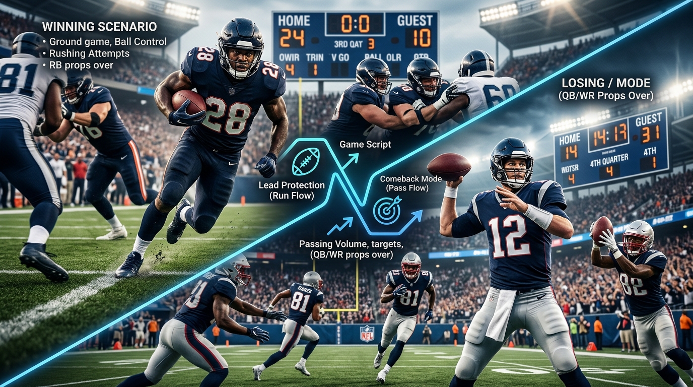
NFL player props are not independent of the game around them. A quarterback does not throw the same number of passes whether his team leads by 10 points or trails by 10. A running back's workload can change when his team is protecting a lead, while wide receivers may see additional targets when their team has to chase points.
That is why NFL player props based on expected game flow require more than looking at a player's season average.
A better approach starts by estimating how the game is likely to develop, then translating those scenarios into player opportunities. The spread, game total, offensive tendencies, matchup, pace, injuries, and coaching decisions all contribute to that forecast. From there, a projection model can estimate how many pass attempts, rushes, targets, receptions, or receiving yards a player is likely to receive.
The important distinction is that expected game flow is not a prediction of exactly what will happen. It is a probability-weighted set of possible scenarios.
Table of Contents
What Expected Game Flow Means for NFL Props
How Game Script Changes Player Volume
Building an Expected Game Flow Projection
Position-by-Position Game Flow Effects
Scenario-Based Player Prop Modeling
Why Game Flow Should Be Modeled as a Distribution
Common Game Flow Modeling Mistakes
How ATSwins Approaches Player Projections
Frequently Asked Questions
Turning Game Script Into Better Player-Prop Projections
What Expected Game Flow Means for NFL Props
Game flow describes the relationship between the score, time remaining, possession, and the decisions teams make as the game develops. In pregame analysis, the objective is not to know the exact score at halftime. It is to estimate the range of game environments that are most plausible.
A betting spread provides one important signal. A sizable favorite is generally expected to have more opportunities to play from ahead, while an underdog is more likely to face situations where passing becomes necessary. The game total adds another piece by describing the expected scoring environment.
Neither number should be treated as a direct player projection.
A team favored by seven points does not automatically produce a running-back over. The favorite could fall behind early, the quarterback could dominate through the air, or the opponent could control possession. Similarly, an underdog quarterback does not automatically throw for a huge number simply because his team is expected to trail.
The better question is:
How does each plausible game state change player opportunity?
This distinction matters because NFL game situations create different incentives as score differentials change. For player props, game flow should therefore be treated as an input to volume rather than a guarantee of production.
How Game Script Changes Player Volume
The clearest effect of game flow is usually volume. Suppose Team A is projected to lead for much of the afternoon. Its offense may have more incentive to emphasize the running game later, especially if the rushing attack is efficient. That can create additional opportunities for running backs as the team attempts to control the clock and protect its advantage. Team B faces the opposite environment. If it spends much of the second half trailing, its offense may need to increase its passing volume, which can lead to more quarterback attempts and additional targets for wide receivers and tight ends.
However, there is a second layer that is easy to overlook: not every player benefits equally from the same game script. In a competitive game, both offenses may maintain a relatively balanced approach, creating more stable volume across their core players. If Team A takes an early lead, its running backs may see more rushing opportunities while Team B's quarterback and receivers could benefit from increased passing volume. If Team B takes the early lead instead, the situation can reverse, with Team A potentially increasing its passing workload while Team B gains opportunities to run the ball.
The scoring environment also matters. A high-scoring game can create more offensive plays and increase passing and receiving opportunities for players on both teams. A low-scoring game can have the opposite effect, while touchdown-dependent props may become more difficult to project because there are simply fewer scoring opportunities available. A large lead late in the game can create another distinct environment, with the leading team potentially becoming more focused on running and clock control while the trailing team becomes more aggressive through the air.
This is why simply comparing a player's season average to a prop line can be misleading. A running back averaging 18 carries per game might project closer to 14 carries in a matchup where his team is expected to trail for much of the afternoon. At the same time, a receiver averaging seven targets could project above that baseline if his team is likely to spend the second half passing to catch up. The player's historical average provides useful context, but it does not necessarily represent his expected workload in every game environment.
A strong player-projection model therefore needs to estimate opportunity first and efficiency second. Game script primarily helps determine how many chances a player is likely to receive, while player efficiency determines what he is likely to produce with those opportunities. Separating these two components makes it easier to understand why the same player can have very different projections from one week to the next, even when his underlying talent has not changed.
Building an Expected Game Flow Projection
A useful game-flow model can start with a relatively small group of inputs.
The first is the expected scoring environment. Team offensive efficiency, defensive efficiency, pace, injuries, weather, and matchup characteristics can all influence expected scoring.
The second is the expected margin. A projected seven-point favorite and a projected one-point favorite should not receive identical game-script assumptions.
The third is each team's tendency to change its play selection based on the score. Some offenses are more willing to continue passing with a lead, while others become more conservative. A model should learn these tendencies from historical play-by-play data rather than assuming every team behaves the same way.
The fourth is player role.
A receiver with a high route participation rate and stable target share responds differently to game flow than a rotational receiver whose playing time is already uncertain. The same principle applies to running backs. A back who handles most early-down and goal-line work has a different projection than one who primarily plays in passing situations.
NFL tracking data can add another layer of information. The NFL's Next Gen Stats system uses player-tracking and event data to produce metrics based on player movements during plays. That type of information can be useful when evaluating player participation, routes, separation, and other elements of performance.
A practical pregame model can therefore work through several layers:
Estimate expected points and margin.
Create multiple plausible score scenarios.
Estimate team pass and rush volume in each scenario.
Allocate that volume among players.
Apply player-specific efficiency assumptions.
Combine the scenarios into a final probability distribution.
That final step is crucial. A model should not simply select one expected game script and pretend it is certain.
Position-by-Position Game Flow Effects
Quarterbacks
Quarterback passing props are among the most directly connected to game script.
A team expected to trail for substantial portions of the game may generate more pass attempts, especially if it reaches the second half needing to close a deficit. That does not automatically mean more passing yards because efficiency, sacks, turnovers, and defensive pressure still matter.
A favorite may also produce a strong passing projection if the matchup encourages aggressive early-down passing or if its offense tends to maintain its normal approach even with a lead.
This is where attempts and yards should be separated.
Game flow primarily affects opportunity. Efficiency determines what the quarterback does with that opportunity.
A quarterback could throw 42 passes and still finish below a passing-yard prop if pressure or coverage forces inefficient throws. Conversely, a quarterback with only 32 attempts could exceed a yardage line if the offense generates explosive plays.
Running Backs
Running-back props often have a strong relationship with positive game script, but the relationship is not universal.
A lead can increase rushing opportunities because offenses may choose to emphasize the ground game while protecting an advantage. However, the magnitude depends on the team's coaching tendencies, offensive efficiency, personnel, and opponent.
A running back can also benefit from negative game script if he is heavily involved as a receiver. That creates an important distinction between rushing props and receiving props.
For a three-down back, a projected deficit does not necessarily make every over unattractive. It may simply shift the player's expected workload from carries toward targets.
This is one reason a complete player projection should separate rushing opportunity from receiving opportunity instead of treating a running back's workload as one number.
Wide Receivers
Wide receivers often benefit from negative game script, particularly when their team has a concentrated passing offense.
But target distribution matters.
If a quarterback throws more frequently, the additional attempts have to go somewhere. A model should determine which receivers are most likely to capture those extra opportunities based on route participation, target share, alignment, personnel usage, and matchup.
A projected high-scoring game can also create a favorable environment for receiving props, but touchdown production remains much more volatile than basic target volume.
A receiver projected for nine targets is not automatically a strong receiving-yard projection. Those targets still need to be converted into catches and yards.
Tight Ends
Tight ends can be more difficult to project because their routes and targets often depend heavily on personnel packages and matchup-specific game plans.
A tight end who stays on the field for most passing situations may benefit from increased pass volume. Another may remain primarily a blocker when the offense expects to run frequently.
That makes route participation and receiving role more informative than simply looking at season receptions.
Scenario-Based Player Prop Modeling
The strongest way to incorporate expected game flow is to model several scenarios rather than relying on one assumed outcome. Imagine a hypothetical game in which Team A is favored by 6.5 points with a projected total of 46. These numbers suggest Team A is expected to score more, but they do not tell us exactly how the game will develop or how that scoring will be distributed. Instead of assuming one specific result, a model can assign different probabilities to several possible game environments. For example, Team A might have a 35% probability of controlling the game, a 40% probability of playing in a competitive matchup, and a 25% probability of falling behind. Under those scenarios, Team A's projected pass attempts could be 31, 35, and 40, while its primary running back could receive 29, 23, and 18 carries. Team B's quarterback might be projected for 38, 35, and 31 pass attempts under those same scenarios. These figures are illustrative modeling assumptions, not historical NFL averages or ATSwins projections.
Suppose Team A's primary running back has an expected rushing efficiency of 4.3 yards per carry. Using the scenario probabilities above, the weighted carry expectation would be calculated as (0.35 × 29) + (0.40 × 23) + (0.25 × 18) = 23.8 carries. If the model expects the player to average 4.3 yards per carry, that produces a baseline rushing projection of approximately 23.8 × 4.3 = 102.3 rushing yards. This approach provides more context than simply looking at a player's season average of 18 carries and 77 rushing yards per game because it considers how his expected workload could change depending on the way the game develops.
The same scenario-based process can be applied to quarterback attempts, receiver targets, receptions, passing yards, rushing attempts, and other player statistics. The important idea is that player opportunity changes with the game environment. A running back may receive more carries when his team protects a lead, while a quarterback and his receivers may see additional passing volume if their team falls behind. By assigning probabilities to different game scripts, the model can create a more realistic distribution of potential player outcomes instead of relying on one fixed projection.
The next step is accounting for correlation between players. If Team A's quarterback throws for 300 yards, the team's receivers are likely to receive a meaningful share of that passing production. On the other hand, if Team A's running back scores twice while the team controls the game, the offense may have less need to maintain aggressive passing volume late in the contest. These relationships mean player props should not always be treated as completely independent events. A quarterback's passing-yard projection is connected to the expected receiving production around him, while a running back's rushing workload is connected to the team's expected scoring environment, offensive efficiency, and likelihood of playing with a lead.
Why Game Flow Should Be Modeled as a Distribution
One of the biggest weaknesses in simplistic prop analysis is treating a projected game script as if it were a single future outcome.
For example:
Team A will win by 10, so its running back will go over.
That statement contains too much certainty.
A better formulation is:
Team A has a higher probability of playing with a lead, which increases the probability of elevated rushing volume for its primary back.
The difference may seem subtle, but it changes the entire modeling process.
A probability-based system can account for several outcomes simultaneously. Team A could win comfortably, win a close game, or fall behind. Each state creates a different distribution of player opportunities.
This approach also makes uncertainty easier to communicate.
If a running back has a projected mean of 21 carries but a wide distribution from 14 to 29, a 20.5-carry line is not automatically an obvious over. The distribution matters.
This is also where calibration becomes important.
Suppose a model repeatedly assigns a 65% probability to a certain type of player prop outcome. If those outcomes occur only 55% of the time over a sufficiently large sample, the model is systematically overconfident.
A strong forecasting process should therefore evaluate not only whether predictions were right or wrong, but whether the probabilities themselves were properly calibrated.
Common Game Flow Modeling Mistakes
The first mistake is treating the point spread as a direct player-prop prediction.
The spread is useful information, but it is not a guarantee of margin. A seven-point favorite can trail throughout the game.
The second mistake is ignoring team-specific tendencies.
Two teams with identical spreads can produce very different player distributions because their offensive philosophies differ.
The third mistake is assuming negative game script always benefits receivers.
A team may fall behind because its offense cannot sustain drives. More passing attempts do not necessarily translate into more receiving yards.
The fourth mistake is ignoring efficiency.
Volume and efficiency are separate variables. A quarterback can throw 42 passes and still finish below a passing-yard line because of pressure, coverage, sacks, or poor completion efficiency.
The fifth mistake is failing to update for injuries.
A missing offensive lineman can change expected efficiency. A missing starting receiver can redistribute targets. A quarterback change can alter the entire passing distribution.
The sixth mistake is overreacting to a single recent game.
A team that ran the ball 35 times last week does not necessarily have a new offensive identity. The model needs enough historical context to distinguish a persistent change from random variation.
Another common mistake is failing to account for correlation between props.
If a model projects a quarterback for unusually high passing volume, that should generally affect the projected opportunities of his receivers. If a team is expected to control the game, that same scenario may reduce the passing volume available late.
Treating every player projection as an independent event can therefore create internally inconsistent forecasts.
How ATSwins Approaches Player Projections
ATSwins treats player projections as probability-based estimates rather than guarantees. Its published player-prop methodology emphasizes contextual information such as historical performance, matchup characteristics, playing time, injuries, pace, and weather rather than relying on one recent box score.
For NFL props specifically, the game-flow concept fits naturally into that framework.
A player projection can begin with the expected team environment, then incorporate the player's expected participation and efficiency. Route participation, target share, rush share, opponent-adjusted efficiency, pressure dynamics, and other NFL-specific signals can then refine the distribution.
This also creates a useful connection between team projections and player props.
If the expected total or spread changes meaningfully, the player distributions may need to change as well.
For example, a late injury could move a team's expected scoring downward while simultaneously increasing the workload of a replacement receiver. Treating those two effects independently can produce inconsistent projections. A connected model is better positioned to recognize that the same piece of news can affect multiple markets.
The practical goal is not to find a player prop that "must hit." It is to estimate the probability distribution accurately enough that a posted line can be evaluated against a reasonable fair expectation.
ATSwins users can also use its broader NFL analytics and player-projection resources as part of that research process, including its NFL advanced stats betting model, AI NFL prediction model, and AI player prop modeling guide.
A Better Workflow for NFL Game-Flow Props
A disciplined workflow is relatively simple.
Start with the team-level forecast. Estimate expected scoring, margin, pace, and offensive efficiency.
Then create multiple game-script branches. Avoid forcing the entire projection through one assumed final score.
Next, estimate how each branch changes pass attempts, rush attempts, and total offensive plays.
After that, allocate opportunities to individual players using role-specific information. A player's expected targets or carries should reflect his participation rate and team structure.
Then apply efficiency estimates. Passing yards require more than pass attempts, just as rushing yards require more than carries.
Finally, compare the resulting probability distribution with the available prop line.
This is where probability becomes more useful than a simple projection.
If a model projects 84 receiving yards, the question is not merely whether 84 is higher or lower than the posted number. The useful question is how often the player should exceed that number under the modeled range of game environments.
That distinction is central to responsible sports forecasting.
Frequently Asked Questions
What does game flow mean for NFL player props?
Game flow describes how the expected score, margin, possession, and clock situation influence team behavior. For player props, it primarily affects opportunity. A team expected to trail may generate more passing volume, while a team expected to protect a lead may generate more rushing opportunities. The exact effect depends on the team's offensive tendencies and the player's role.
Which NFL player props are most affected by game script?
Passing attempts, rushing attempts, targets, receptions, and passing or rushing yards can all be affected. Touchdowns are also influenced by scoring environment, but they are more volatile because a small number of red-zone opportunities can determine the result. The strength of the game-flow relationship varies by player role.
Should NFL favorites automatically lead to running-back overs?
No. A favorite is more likely to play with a lead, which may increase rushing opportunities, but the relationship is not automatic. Offensive philosophy, matchup, quarterback tendencies, early-game performance, and the possibility of a competitive game all matter. A running back who contributes heavily as a receiver may even retain strong opportunity in negative game scripts.
How do sportsbooks account for expected game flow?
Player prop pricing incorporates many sources of information, and the exact methodology used by individual sportsbooks is not public. A bettor or modeler should therefore avoid assuming that one variable, such as the spread, represents the entire market expectation. Game total, team tendencies, injuries, matchup, player role, and the current price all belong in the analysis.
Can AI improve NFL game-flow prop projections?
AI and statistical models can process many variables simultaneously and estimate probabilities across multiple scenarios. They do not eliminate uncertainty. Good models still need clean data, time-aware validation, calibration, injury updates, and safeguards against overfitting. The objective is better probability estimation, not certainty.
Turning Game Script Into Better Player-Prop Projections
The most useful way to think about NFL player props based on expected game flow is to stop treating the prop as an isolated number.
A quarterback's passing projection depends partly on how often his team is expected to throw. A running back's rushing projection depends partly on whether his team is expected to control the game. A receiver's target projection depends partly on how much passing volume his offense is likely to generate and how those targets are distributed.
That does not mean the game script will unfold exactly as projected. Football contains too much variance for that. The value of the model comes from estimating several plausible paths and weighting them appropriately.
ATSwins approaches this type of analysis through data, projections, probabilities, and contextual factors rather than guarantees.
For readers building their own NFL prop process, the most important takeaway is simple:
Project the game environment first, then project the player inside that environment.
That framework produces a more coherent estimate of opportunity and gives player props a stronger analytical foundation than season averages alone.