

How to Calibrate Sports Probability Models and Test Forecast Reliability
A sports probability model is only useful if its probabilities mean what they say. If a model assigns a basketball team a 70% chance of winning across many comparable games, that group of teams should win approximately 70% of the time for the model to be well calibrated. Individual results will vary, but repeated forecasts should match their stated likelihoods reasonably closely.
Sports probability model calibration is the process of measuring and, when necessary, correcting the relationship between predicted probabilities and observed outcomes. It answers a different question from prediction accuracy: not simply whether a model picked the winner, but whether its confidence was justified.
For sports analytics platforms such as ATSwins.ai, that distinction matters when evaluating game forecasts, fair-line estimates, simulations, and player projections. A disciplined calibration process uses historical predictions, time-aware testing, appropriate scoring rules, and enough observations to separate meaningful patterns from ordinary sports variance.
What Sports Probability Calibration Means
Probability calibration measures whether forecast probabilities correspond to the frequency of events that actually occur.
Imagine a model that produces 1,000 predictions, each assigning a team a 60% chance of winning. If approximately 600 teams win, the model's forecasts are well calibrated at that probability level. If only 480 win, the model may be systematically overconfident. If 720 win, it may be underconfident.
These comparisons must be made across a sufficiently large, relevant set of forecasts. A 60% prediction that loses is not automatically a bad prediction. Its implied loss probability was 40%, so losing was always a realistic possibility.
Calibration is also different from discrimination. Discrimination describes how effectively a model distinguishes more likely winners from less likely winners. Calibration describes whether the probabilities assigned to those outcomes are numerically trustworthy.
A model may rank stronger teams above weaker teams while consistently overstating their chances. Another may produce reasonable probabilities but struggle to distinguish close matchups. Those are different problems, and they call for different solutions.
Sports models also require care about what event is being predicted. A moneyline win, a spread cover, an over, and a player exceeding a statistical threshold are separate targets. A model calibrated for game winners is not automatically calibrated for player props or totals.
For a broader introduction to how probabilities are generated, see ATSwins.ai's article on sports outcome forecasting and probability estimation.
Why Accuracy Is Not Enough
Classification accuracy counts correct and incorrect predictions after a probability is converted into a decision. For example, a model might select the home team whenever its win probability exceeds 50%.
That approach discards information. A forecast of 51% and a forecast of 90% both count as one correct prediction if the team wins. Yet they express very different levels of confidence.
Consider two models evaluated on the same 100 games. Model A predicts 60% for a group of evenly matched games and gets 60 winners correct. Model B predicts 85% for those same games but also gets 60 winners correct.
Their accuracy is identical. Their probability quality is not. Model B is claiming substantially more certainty than its outcomes support.
A 2024 study, Machine learning for sports betting: Should model selection be based on accuracy or calibration?, investigated this distinction using NBA data and historical odds. Its reported experiments support evaluating probability calibration rather than selecting models solely by classification accuracy. The findings are evidence from a particular research design, not a guarantee that calibration alone will improve financial returns in every setting. See the published study.
The practical lesson is straightforward: evaluate the quality of the probability itself, not just the final winner label.
How to Measure Calibration
No single statistic fully describes a sports forecasting model. Strong evaluation combines visual diagnostics, proper scoring rules, and out-of-sample testing.
Reliability diagrams
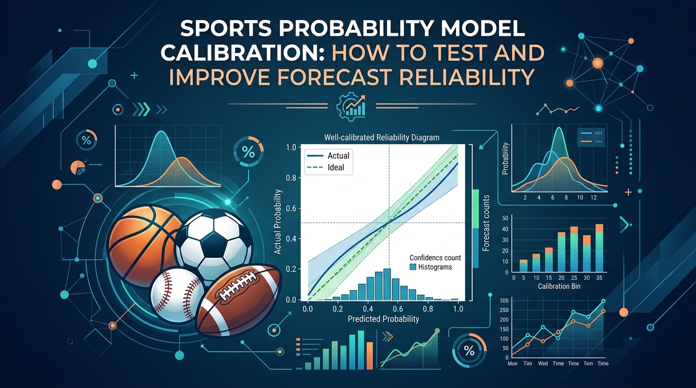
A reliability diagram, also called a calibration curve, groups forecasts into probability ranges and compares their average predicted probability with the observed event frequency.
For example, suppose a group of NFL forecasts averages 65% probability of a home win. If home teams in that group win 58% of the time, the model is overestimating the outcome frequency at that level.
A well-calibrated model tends to produce points near the diagonal line where predicted probability equals observed frequency.
The direction of the error matters. Points below the diagonal indicate overconfidence for the event being measured; points above it indicate underconfidence. Analysts should also examine how many forecasts fall into each range. A curve based on a handful of games may look dramatic without providing strong evidence of a persistent problem.
The scikit-learn probability calibration documentation explains reliability diagrams and how to calculate them.
Brier score
The Brier score measures the squared difference between a predicted probability and the actual binary outcome. For a forecast probability pi and result yi, where a win is 1 and a loss is 0, the score is:
Brier Score = (1/N) × Σ(pi − yi)²
Lower scores are better when comparing appropriate datasets for the same prediction task.
Suppose a model assigns a team a 70% chance to win. If the team wins, the squared error is (0.70 − 1)² = 0.09. If it loses, the error is (0.70 − 0)² = 0.49.
The second result produces a larger penalty, but that does not mean the original prediction was unreasonable. A probability forecast is evaluated over many events, not judged entirely by one outcome.
The Brier score captures several aspects of probabilistic forecast quality, including calibration and the ability to distinguish events with different likelihoods. It should not be treated as a pure calibration measurement in isolation.
Log loss
Log loss penalizes probability forecasts according to how much probability they assign to the outcome that occurs. It places particularly strong penalties on confident forecasts that are wrong.
That makes it useful for identifying a model that routinely assigns extremely high probabilities to outcomes that fail to occur. However, extreme probabilities and small samples require careful handling.
Calibration error and sample size
Expected calibration error (ECE) summarizes the difference between predicted and observed frequencies across probability bins. It can provide a convenient diagnostic, but its value depends on how bins are defined and weighted. Different implementations may produce different results.
For a more complete review, compare a reliability diagram with Brier score and log loss. Also include a simple baseline model. A sophisticated model should demonstrate improvement against a meaningful reference, not merely produce an attractive chart.
A Worked Sports Calibration Example
Consider a hypothetical model that predicts NBA home-team wins. After recording predictions and results from a held-out evaluation period, an analyst groups forecasts into probability bands.
| Average predicted probability | Observed home win rate | Initial diagnosis |
|---|---|---|
| 50% | 51% | Close to calibrated |
| 60% | 54% | Overconfident |
| 70% | 61% | Overconfident |
| 80% | 66% | Substantial overconfidence |
Illustrative figures only; this is not a report of ATSwins.ai performance or a real sports dataset.
The pattern suggests that high-confidence forecasts are too aggressive. The analyst should first check the number of games in each band and whether the error persists across seasons, teams, and different market conditions.
If the pattern is stable, a calibration method may adjust the raw model outputs. A raw 80% forecast might be mapped to a lower calibrated probability, for example. The exact adjustment must be learned from historical calibration data and then tested on separate observations; it should not be chosen simply to make the displayed curve look better.
That correction also changes how a model's probabilities translate into fair odds.
For decimal odds, the simplest fair-price conversion is:
Fair decimal odds = 1 / p
A calibrated 60% probability implies fair decimal odds of approximately 1.67, before accounting for any bookmaker margin or other pricing considerations. A 50% probability implies fair decimal odds of 2.00.
The difference between a model probability and a market-implied probability is only a starting point for analysis. Price availability, margin removal, uncertainty, and the quality of the underlying estimate still matter. A calibrated forecast does not guarantee that a market offers value.
How to Improve Model Calibration
Calibration should follow a repeatable process rather than a series of manual adjustments made after disappointing results.
First, preserve the original forecast. Record the predicted probability, event definition, timestamp, model version, relevant inputs, and final result. Without this history, analysts cannot reliably reconstruct what the model knew before a game began.
Second, divide data by time. Train the underlying model on earlier games, fit the calibration layer on a separate later period, and evaluate the finished pipeline on still later data. Random splits can create misleading results when sports data contains time trends or when information from the same teams and seasons crosses between sets.
Third, choose a correction method appropriate to the amount and shape of the available data.
Platt-style or sigmoid calibration fits a smooth mapping between model scores and observed outcomes. It is relatively compact and may be useful when data is limited, although it cannot correct every possible distortion.
Isotonic regression learns a flexible, non-decreasing mapping. It can capture more complex calibration patterns but may overfit when the calibration sample is small. The scikit-learn documentation discusses these trade-offs and provides implementation guidance.
Temperature scaling is another option for multiclass models, including forecasts that assign probabilities to home win, draw, and away win. It adjusts the sharpness of predicted class probabilities without changing their ranking under the standard formulation.
The method should be selected based on validation performance rather than complexity or popularity.
After fitting the calibrator, evaluate the entire system on untouched data. Compare calibration curves, Brier score, log loss, and performance against the original model. Check whether any apparent improvement survives across different time windows and relevant subgroups.
Finally, monitor calibration after deployment. A correction that works early in a season may weaken when team personnel, coaching strategies, league scoring environments, or model inputs change. Recalibration should be triggered by evidence of drift, with enough recent observations to support the adjustment.
Common Calibration Mistakes
The most damaging error is data leakage: using information that would not have been available when a prediction was made. Examples include joining a historical game to a later injury report, using final statistics as pregame features, or fitting the calibration layer on the same outcomes used to report final performance.
Another mistake is treating every sport or market as interchangeable. Football game outcomes, baseball totals, hockey moneylines, and player rebound props have different base rates and sources of uncertainty. Calibration should be evaluated for the specific target, with pooling across groups used only when statistically justified.
Overreacting to a short run of losses is equally dangerous. Even a calibrated 70% forecast loses 30% of the time in expectation. A few losses do not prove that a model is broken, just as a winning streak does not establish that its probabilities are accurate.
Analysts should also avoid selecting probability bins so aggressively that each contains too few events. Sparse bins produce noisy observed frequencies, especially near 0% and 100%. Confidence intervals, rolling evaluation windows, and sensible aggregation help show how uncertain the calibration estimate itself may be.
Finally, calibration is not the same as profitability. A forecast can be well calibrated and still offer no advantage at available market prices. Transaction costs, bookmaker margins, price movement, and model uncertainty all affect the practical value of a forecast.
Applying Calibration to Sports Forecasting
For a platform that produces game projections, simulated outcomes, player estimates, and fair-line numbers, calibration connects the modeling layer to the decision layer.
ATSwins.ai describes its platform as providing model-based win probabilities, projected totals, spread expectations, simulation outputs, fair-price estimates, and market comparisons. These outputs create different evaluation questions: do game probabilities match observed win rates, do simulated scoring distributions reflect real scoring patterns, and do player estimates perform appropriately for their intended use?
The validation target must match the output. A binary win probability can be assessed using reliability diagrams and proper scoring rules. A projected point total requires evaluation of numerical error and, where available, the quality of its predicted distribution. A player projection also needs to be judged against its exact target, with special attention to minutes, role changes, injury status, and opponent context.
Calibration should be paired with a disciplined record of the market price and the time a forecast was issued. Closing-line value (CLV) can provide a separate view of how an estimated price compares with a later market price, but it does not replace calibration or prove that a forecast is correct.
Readers interested in the broader modeling workflow can review ATSwins.ai's guide to building a sports probability model and its explanation of sports analytics software and model evaluation.
The key is transparency: preserve the forecast as originally issued, distinguish model estimates from actual results, and report evaluation periods clearly. A model's current output should not be presented as proof of long-term reliability unless appropriate historical testing supports that claim.
Putting Calibrated Probabilities to Work
Sports probability model calibration gives analysts a way to test whether forecast confidence is deserved. It moves evaluation beyond winner-picking accuracy and toward a more useful question: when a model says an event has a particular chance of occurring, do comparable events occur at roughly that rate?
The strongest process combines reliable data, time-aware validation, calibration curves, proper scoring rules, and ongoing monitoring. It also recognizes the limits of the evidence. Injuries, tactical changes, random variance, and market movement can all affect results, and a calibration adjustment cannot remove those uncertainties.
For ATSwins.ai readers, the practical objective is to evaluate projections and fair prices with more discipline rather than treating any single forecast as a certainty. Explore the platform's sports forecasting and market-analysis resources alongside a documented evaluation process, and judge the quality of a model by its sustained performance on data it did not train on.
Frequently Asked Questions
What is calibration in sports prediction models?
Calibration measures whether predicted probabilities correspond to observed outcome frequencies. If a model issues many 60% win forecasts, roughly 60% of those outcomes should occur over a sufficiently large and relevant sample. Calibration does not require every individual prediction to be correct. It evaluates the consistency between stated probabilities and results across groups of forecasts.
What is the best metric for sports probability calibration?
There is no single best metric for every purpose. Reliability diagrams show where forecasts are overconfident or underconfident, while Brier score and log loss measure overall probabilistic forecast quality. Expected calibration error can provide a summary, but it depends on binning choices. Using multiple measures and a meaningful baseline provides a more complete evaluation than relying on one number.
Can a model be accurate but poorly calibrated?
Yes. A model can correctly identify many winners while assigning probabilities that are too high or too low. Accuracy evaluates categorical decisions; calibration evaluates the numerical probabilities behind those decisions. A model that predicts 80% for events that occur only 65% of the time may still rank teams well, but its confidence estimates need investigation.
How often should a sports model be recalibrated?
There is no universal schedule. Recalibration should depend on evidence of drift, the volume of new data, and the stability of the sport and market being modeled. Analysts should monitor performance over time and avoid making large adjustments from a small number of games. Any updated calibration method should be evaluated on data not used to fit it.
Does good calibration guarantee profitable sports bets?
No. Calibration measures probability reliability, not profitability. A well-calibrated model may agree with market prices and provide no advantage after bookmaker margin and other costs. Practical evaluation also requires comparing estimated probabilities with available prices, accounting for uncertainty, and reviewing results over a meaningful sample without assuming that past performance will continue.