

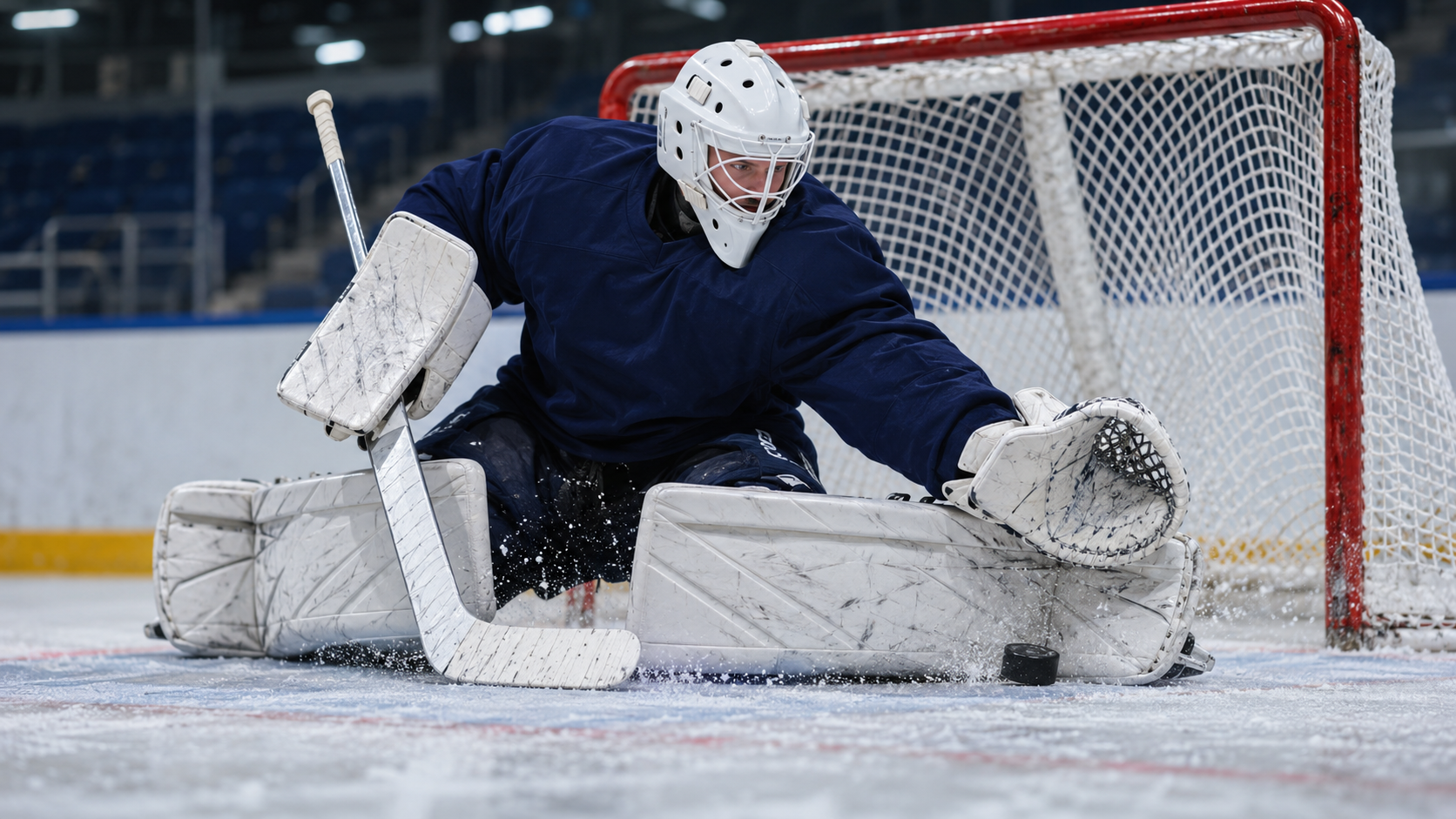
An NHL goalie saves prediction model estimates how many shots a goalie will stop by forecasting the shots he will face, his probability of stopping them, and how long he will stay in net. A useful starting point is expected shots against multiplied by an expected save rate. The next step is estimating the range of possible save totals.
That second step is where the analysis gets interesting. A projection of 28 saves does not tell you the chance of clearing 27.5, and a strong goalie does not automatically produce a high save total. Workload matters. This article walks through a practical modeling approach, a transparent probability example, and the checks that keep a precise looking forecast from outrunning the information behind it.
Start With the Stat You Actually Want to Predict
A goalie’s save total is the number of shots on goal he stops. For shots credited against that individual goalie, saves equal shots against minus goals allowed. Use the goalie’s own workload rather than blindly subtracting the team’s final goals allowed from its shots against, especially when multiple goalies appear or an empty net is involved.
Attempts that miss the net or are blocked before reaching the goalie do not become saves. That makes opponent shot attempts a useful input rather than the final forecast target. A team can spend long stretches attacking without forcing the goalie to stop every puck it directs toward the net.
Save percentage measures stopping efficiency, while total saves measure a combination of efficiency and opportunity. Imagine one goalie stops 23 of 25 shots and another stops 32 of 36. The first has the higher save percentage, but the second makes more saves. For a saves projection, the workload difference cannot be brushed aside.
Keep the market definition attached to the data. Confirm whether the offered total includes overtime and how participation, replacements, and statistical corrections are handled. Use the same scope when training and evaluating the model. A forecast and a market line are only comparable when they describe the same event.
Build an NHL Goalie Saves Prediction Model in Two Stages
Begin by estimating shots on goal against during the goalie’s expected time in net. Blend the opponent’s attacking volume with the defending team’s shot suppression, while accounting for schedule strength and manpower situations. Simply averaging two raw per game numbers is a baseline, not proof that the matchup has been modeled well.
Separate even strength and special teams when the data supports it. A hypothetical forecast might assign 25 shots against at even strength and six during other included situations, for 31 total. Those numbers are invented teaching inputs, not live team statistics. Their purpose is to show where the total comes from.
Next, estimate the stopping probability for those shots. Multiplying 31 expected shots by an assumed 0.910 save rate gives 28.21 expected saves. This is a transparent approximation under a fixed rate assumption. In a richer model, shot difficulty and game conditions can change both workload and the probability of a save.
Do not assume the product of two averages always equals the average of their product. If high volume scenarios also bring harder chances or an earlier goalie exit, the relationship matters. Simulating workload and shot difficulty together is one way to preserve those connections instead of pretending the inputs are independent.
Machine learning might estimate the workload, the stopping probability, or the save total directly. Each approach still needs a baseline comparison and clear input timing. A complicated model that cannot outperform a simple shot volume forecast on later games has not earned extra trust just because it uses more variables.
Give Shot Volume and Playing Time Their Own Attention
A small workload revision can matter more than a noticeable change in save rate. At 31 expected shots, moving the assumed stopping rate from 0.900 to 0.920 changes expected saves from 27.90 to 28.52. Holding the rate at 0.910 while moving expected shots from 28 to 34 changes expected saves from 25.48 to 30.94.
That comparison is arithmetic under hypothetical assumptions, not a claim that workload always dominates in every matchup. It does explain why starting with a goalie’s reputation misses much of the problem. A strong defensive team might protect an excellent goalie so well that he has little opportunity to reach a high total.
Confirm the starter before treating a named goalie projection as actionable. Before confirmation, keep forecasts conditional: one estimate if goalie A starts and another if goalie B starts. Combining them without labeling the assumption can produce a number that describes neither player’s likely assignment.
Playing time requires similar care. Being pulled for an extra attacker late in a game removes opportunities, while replacement after an injury or a difficult start can sharply reduce exposure. A full game assumption may be useful as a baseline, but its limits should be visible. Do not invent a precise early exit probability without evidence.
Shot quality also belongs in the workload discussion. Perimeter shots and dangerous chances near the net need not have the same stopping probability. A forecast that expects more difficult chances should reflect that mix rather than applying the goalie’s recent overall save percentage to every matchup unchanged.
Turn Expected Saves Into an Over Probability
Consider a deliberately simple teaching model. Suppose shots faced follow a Poisson distribution with a mean of 31, and every shot has an independent 0.910 chance of being saved. Assume the goalie remains in net throughout the modeled exposure. Under those assumptions, saves follow a Poisson distribution with a mean of 28.21.
For over 27.5 saves, the relevant event is at least 28 saves. Its probability is one minus the combined probabilities of zero through 27 saves. Calculating that sum gives approximately 54.09%. The mean of 28.21 sits above the line, but the chance of clearing it is much closer to a coin flip than the raw comparison might suggest.
This distribution is a teaching choice, not a claim that actual goalie workloads are Poisson. A model that fixes shots faced at exactly 31 would instead give a binomial save distribution under the same independent stopping assumption. Those models share the same expected saves but have very different spreads because only one lets workload vary.
Real games add uncertainty around penalties, possession, shot quality, and playing time. A count model with extra dispersion or a simulation of different game conditions may describe the results better. Select the approach using held out games and probability checks, rather than picking whichever distribution produces the most appealing over percentage.
The useful question is therefore how a model produced its probability. An average alone leaves too much unknown. Ask whether the model allows a quiet night, a busy night, and an interrupted appearance, and whether their relative frequencies resemble what happens in comparable games.
Compare the Forecast With a Price, Not Just a Line
Suppose a separate hypothetical model estimates a 56% probability of at least 28 saves. Its fair decimal odds are 1 divided by 0.56, or about 1.79. Fair odds express that estimate without adding a bookmaker margin. They are a translation of an assumption, not a guarantee that the estimate is correct.
At an available decimal price of 1.90, break even is about 52.63%. Using the assumed 56% probability, expected net return per unit is 0.56 multiplied by 1.90, minus one, or 0.064. That is 6.4% per unit mathematically, conditional on the estimate. Actual short term outcomes can look nothing like that average.
Now reduce the estimated probability to 52% after revising the expected workload. The same calculation becomes negative 1.2% per unit. Nothing about the offered price changed. The conclusion flipped because the information supporting the forecast changed, which is exactly why sensitivity checks deserve a place before any decision.
When comparing the model with the market, inspect both over and under prices at the same threshold and account for the margin. Over 27.5 and over 28.5 are different events. Keep a record of the actual threshold and price available when the forecast was evaluated, rather than comparing against whichever closing quote looks best afterward.
Use Recent Form Without Letting a Few Starts Take Over
Recent saves can tell you that a goalie has been busy, but the total does not explain why. A run of difficult opponents, repeated penalty kills, or unusual overtime exposure might be responsible. Review those conditions before deciding that the next game deserves the same workload projection.
Save percentage needs sample size context too. A few goals have a large effect when the number of shots faced is small. A sensible estimate blends recent evidence with a broader baseline, using a method that has been tested on future games. The amount of blending should be justified rather than chosen because it makes a preferred player look better.
Team changes can make older information less representative. A different defensive lineup, coaching approach, or penalty killing role may change the shots a goalie faces. Update the relevant input and acknowledge uncertainty when the new arrangement has barely played together. More recent data is useful when it describes a real change, not merely because it is recent.
For context, ATSwins NHL player props and NHL game projections provide relevant places to begin player and matchup research. The examples in this article are independent teaching calculations. They do not describe proprietary ATSwins formulas, live probabilities, or a verified record for goalie saves.
Test the Model on Games It Has Not Seen
Split the data chronologically. Train using earlier games, generate forecasts for later games, and move forward without using information that arrived after the prediction. Final starting assignments, revised statistics, and end of season averages can quietly leak future information into a backtest if their timing is ignored.
Measure average error for save totals, then compare it with simple baselines over the same games. Inspect whether the model systematically overestimates low workload matchups or underestimates busy ones. A reasonable overall average can hide mistakes that repeatedly affect one type of goalie appearance.
Evaluate threshold probabilities separately through calibration. Among many forecasts near 60%, roughly 60% should clear the stated threshold, allowing for sampling variation. A model can predict average saves reasonably well while assigning poor probabilities because it underestimates the range of outcomes. Track the distribution, not only its center.
Historical profit is another measure with different requirements. It needs realistic available prices, consistent settlement rules, and a fixed selection process. A favorable closing price can provide useful evidence about market timing, but it does not establish that a model is calibrated or profitable. Report the sample size and avoid treating a brief winning stretch as a durable advantage.
Questions About Goalie Saves Forecasts
Does the better goalie usually have the higher saves projection?
Not necessarily. Goalie ability affects the fraction of shots stopped, while team defense and opponent attack shape how many shots arrive. A weaker goalie facing a much heavier workload can have the higher expected total. Compare both components before ranking projections, and keep efficiency separate from the number of opportunities to make a save.
Is a projected total of 29 enough to take over 28.5?
No. You still need the probability of at least 29 saves and the available odds. The mean does not reveal the shape of the outcome distribution. An uncertain workload or a meaningful chance of reduced playing time can change that probability considerably. A half save gap between the average and the line does not establish value.
What should change after a late starter announcement?
Recheck the named goalie, expected playing time, stopping estimate, and the posted market. The opponent’s attacking strength might stay the same, but the personnel assumption has changed. Confirm the revised forecast has a fresh timestamp. If the starter news conflicts with the displayed projection, wait for a consistent set of inputs rather than mixing old and new information.
Make the Workload Assumption Easy to Challenge
A forecast becomes easier to judge when you can explain why the goalie is expected to face a particular number of shots. Write down that workload, the stopping assumption, and the conditions under which the estimate would change. Then test the input you trust least before putting weight on a small price difference.
Keep the result useful even when it leads to no action. An unclear starter, a stale timestamp, or a forecast that changes dramatically under plausible conditions is a reason to wait. That is a valid outcome of disciplined analysis.
For broader game pricing context, review the ATSwins NHL Oddsmaker page alongside the player forecast. Keep the probability, threshold, and available price together, and use the next result to improve your assumptions rather than judge the entire process from one night.