

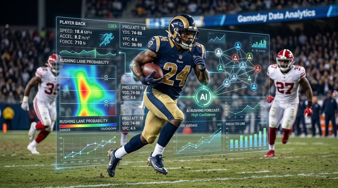
Every single week, I take raw play-by-play data, coaching tendencies, and Friday injury reports, and I turn them into clear projections using AI. It is not magic, it is just a solid method. In this guide, I am going to show you exactly how I forecast rushing attempts with context that actually matters, like game pace, personnel groupings, weather conditions, and specific matchups. You can expect plain talk, transparent steps, and numbers you can trust for smarter bets and fantasy calls.
Table Of Contents
Problem framing and data ingestion
Feature engineering and target leakage control
Modeling approaches and training
Validation, backtesting and calibration
Forecast workflow, deployment and communication
Conclusion
Related Posts
Frequently Asked Questions (FAQs)
Building an NFL Rushing Attempts Projection Model That Bettors Can Trust
Problem framing and data ingestion
Define the target clearly before writing code Before you type a single line of code or train any model, you need to be totally explicit about what you are projecting. For rushing attempts, there are a few consistent targets that map cleanly to betting markets and internal decision-making processes. You have player rushing attempts per game, which is the big one. Then you have player rushing attempts per neutral-script quarter, which is possession-weighted for when the game is tied or within seven points. You also have team rushing attempts per 60 offensive plays to normalize for overall pace. Beyond those, you can look at running back room rushing attempt shares, like how carries break down between your primary back, secondary back, quarterback, and wide receivers. Finally, you have short-yardage carries on three yards to go or less, which helps a ton if you are building role-specific prop models.
You should pick one primary target and one normalization target. For spread betting and player prop use-cases, I always recommend using player rushing attempts per game as the main output that bettors actually care about. Then, use carries per 60 plays and carries per neutral-script quarter as calibration layers. These layers let you check for drift and produce scenario-specific forecasts. Make sure every single target is game-joinable by team, opponent, week, and player identification number, and ensure that you can compute it with zero leakage from future weeks.
Scope seasons and games deliberately The regular season should always be your baseline dataset. You should only include playoff games if you are also planning to forecast the postseason, but it is usually best to keep them separate because usage patterns and rotation depth change materially when teams are playing for their lives. Three to five recent seasons will capture current league-wide offensive tendencies while balancing scheme stability across coaching changes. You want to exclude games with extreme outliers when they are clearly data errors, but you definitely want to keep blowouts because blowout scripts reflect real-world coaching behavior under stress. Document every filter you set up. If your model is going to be used on ATSwins, logging your data filters is a core part of maintaining reproducibility and keeping things reliable.
Core data sources and what they cover For play-by-play data, I lean heavily on nflfastR play-by-play datasets via nflverse. This gives you down, distance, time, score differential, play type, rusher identification, formation and personnel tags, penalties, and success indicators. For roster and injury information, you can use nflverse weekly roster merges alongside inactives files, supplementing them manually if something looks off. For snap counts and overall usage, Pro-Football-Reference provides solid team pages and game logs to track snap shares, touches, and rolling usage trends. For weather and surface details, you want to track stadium roof types plus historical weather feeds covering temperature, wind, and precipitation. If you do not have a paid commercial weather feed, you can easily create a lightweight proxy using known stadium attributes and public weather archives. If you want advanced context, box counts and alignment data from NFL Next Gen Stats are awesome for validation or calibrating your proxies.
Building a reliable ingestion flow To set up a flow that does not break, start by pulling weekly play-by-play data for all games in your target scope and saving it in a partitioned store organized by season and week. Next, join your rosters to ensure every rusher identification number maps cleanly to player metadata like position, team, and tenure. Layer in snap counts from Pro-Football-Reference, aligning them by team, game date, and player to eliminate mismatches. Then, create a clean canonical keys schema. Your game key will use season, week, and game identification numbers. Your team perspective key uses offense team, defense team, and home or away status. Your player perspective key tracks player identification, position, depth chart slot, and jersey number. Finally, log every step of the ingestion process by recording the total number of games, total players, duplicates resolved, and the percentage of plays that have valid personnel tags.
Data hygiene checklist Always deduplicate plays right out of the gate. Duplicates are pretty rare in play-by-play data, but you will occasionally run into replayed downs or complex penalty sequences that double-count. Next, validate that total carries logged by a team equal the sum of individual player carries for that game. Confirm that team play totals equal the sum of all play types plus penalties and aborted snaps. If you find missing personnel tags, fill them with an unknown label and build a dedicated data-quality feature so your model knows when a play is missing details.
Feature engineering and target leakage control
Situation-neutral run rate and script-aware features Situation-neutral run rate represents the percentage of offensive plays that are runs when the score is within seven points and the time remaining is outside of the two-minute warning in either half. Early-down tendencies are also huge, specifically run rates on first-and-ten and second-and-medium. These numbers act as strong indicators of a head coach or offensive coordinator's underlying DNA. You should also isolate short-yardage run inclination on three or fewer yards to go, along with goal-line run share inside the five-yard line. Tracking carries inside the five by position group massively improves your player role projections.
Rolling windows keep your features fresh. I recommend setting up team rolling four-week and season-to-date run rates. You should also track a coach's rolling profile across different teams if they changed jobs recently. On the player side, look at rolling usage metrics like attempts per game, rush share of team attempts, overall snap share, and inside-the-five attempts.
Coach, scheme, and offensive line proxies For coaching history, look at head coach and offensive coordinator run-pass splits normalized against the current league average for that season. For personnel reliance, track the share of total plays run out of 11, 12, and 21 personnel groupings, and calculate the run rate within each specific group. For offensive line run-blocking proxies, you can pull Adjusted Line Yards or similar public metrics. If those are not directly available in your pipeline, you can derive proxies by looking at stuffed run rates allowed versus created, penalties drawn or committed on the line, and the success rate on interior rushes compared to edge rushes. Offensive line continuity is another massive signal. A simple count of returning starters from zero to five serves as a strong baseline input.
Quarterback rush share and designed versus scramble splits Separating a quarterback's designed running attempts from their scramble attempts helps you avoid artificially inflating running back projections for teams with mobile quarterbacks. High scramble volume usually replaces pass attempts, not handoffs. You also need to track quarterback kneel and sneak shares because those plays siphon high-probability short-yardage and game-ending attempts directly away from the running back room.
Pace and play volume Neutral-script pace measures the average seconds per play when a game is competitive. Combine this with no-huddle rates and the average number of plays generated per drive. You also need to factor in opponent pace so your model can anticipate the total play volume environment for both teams involved in the matchup.
Weather, surface, and stadium impact Surface type matters. Playing on field turf versus natural grass, or inside a dome versus outdoors, impacts running tendencies over time. In cold, windy, or wet conditions, teams tend to ground the ball more often. You can group weather into distinct bins for temperature, like under 35 degrees, 35 to 55 degrees, and over 55 degrees. For wind, bin it into zero to 10 miles per hour, 10 to 20 miles per hour, and over 20 miles per hour. Add a simple flag for active precipitation. Interaction terms are super useful here. A windy, outdoor, late-season game almost always nudges a coaching staff toward a higher overall run rate.
Box counts and front alignment If you have access to NFL Next Gen Stats, you can track stacked box rates (eight or more defenders in the box) and light box rates (six or fewer defenders). These numbers correlate directly with per-carry success and how coaches allocate run attempts. If you do not have Next Gen Stats, you can approximate these variables by tracking opponent safety depth, base versus nickel defense frequency, and run-stop personnel packages pulled from play-by-play tags. Look at opponent front types too. Identifying odd versus even fronts gives you a solid lens into whether a team relies on gap or zone schemes and how stable a running back's role will be.
Injuries and inactives (and how not to leak future info) Injury news drops on multiple timelines throughout the week, so you must build features using only information that was officially known at your specific forecast lock time. Track practice participation trends from Did Not Practice to Limited and Full across Wednesday, Thursday, and Friday. Official inactives drop 90 minutes before kickoff, but if you are projecting earlier in the week, you need to use injury probabilities and multi-scenario outputs.
When it comes to depth chart adjustments, if a primary running back carries a Questionable tag after a midweek downgrade, you should widen the variance on the running back room share and create distinct scenario branches. Do not forget about special teams workload either. Heavy special teams snaps for a backup running back usually put a hard cap on their potential offensive carries.
Travel, rest, and schedule density Track rest days since the last game along with bye-week boosts. Total travel miles and time zones crossed are also worth monitoring, as long cross-country trips occasionally distort early-game offensive script and player rotations. Finally, flag short weeks like Thursday Night Football games alongside international slate travel.
Lag structure and rolling windows that prevent leakage To keep your data completely clean, make sure your rolling windows strictly use past weeks. If a player gets traded or changes teams mid-season, reset their rolling windows unless they are moving with a coach or scheme they previously played under. For high-profile rookies entering the league, apply priors built from their college usage metrics translated through historical positional comps. Then, systematically decay those priors as real NFL data accumulates over the first few weeks of the season.
A lightweight feature store template To organize your data pipeline cleanly, you can set up a unified feature store schema. Your core entity keys will include season, week, team identification, player identification, opponent identification, and home or away status. Your target feature windows should include:
Team neutral run rate over a four-week rolling window Early-down run rate season-to-date RB1 snap share over four weeks RB2 snap share over four weeks Quarterback designed run share season-to-date Personnel 11 run rate season-to-date Personnel 12 run rate season-to-date Neutral pace over four weeks Opponent neutral pace over four weeks Weather category bin Surface type Offensive line starter continuity count Adjusted line run proxy score Injury status active probability Injury status limited probability
Your final target labels will focus on player attempts per game, team attempts per 60 plays, and neutral attempts per quarter.
Modeling approaches and training
Start with simple, transparent baselines I always recommend starting with simple Poisson regression for counts at the player-game level, using the natural log of expected plays as an offset. If the variance in your target data exceeds the mean by a significant margin, step up to a Negative Binomial model and tune the dispersion parameter. These simple baselines show you right away whether your custom features are actually adding predictive signal beyond basic play volume and game script.
Regularized GLMs for interpretability L1 and L2 regularized Poisson or Negative Binomial models work incredibly well when you need total interpretability for player attempts. You can set total offensive plays or neutral-script plays as your offset. Your key predictors will include team neutral run rate, early-down run tendency, running back snap share, opponent light-box rate proxies, weather bins, point spread, and game total.
The main advantage of regularized GLMs is that the coefficients are completely transparent and readable for analysts, making them perfect for explaining player prop bets. The main downside is that they have trouble handling complex non-linear relationships, meaning you have to manually engineer every single interaction term yourself.
Tree ensembles in scikit-learn for nonlinearity Gradient Boosted Trees and Random Forests built in scikit-learn excel at automatically capturing non-linear patterns. They pick up tricky interactions between weather, spread, pace, and personnel groupings. They also handle threshold effects cleanly, like how a point spread opening wider than seven points changes a team's offensive script entirely.
When training tree ensembles, always use stratified time-based splits instead of random cross-validation. Keep a close eye on feature importance drift week over week. To get reliable outputs, calibrate your predictions by mapping the model's predicted means directly to integer count distributions using Poisson mixtures or post-hoc rounding adjustments.
Hierarchical Bayesian models in PyMC for partial pooling If you want to handle thin samples and uncertainty like a pro, build a hierarchical Negative Binomial model in PyMC. This approach uses partial pooling across multiple levels of your dataset, including team-level run identities, individual player talent and role profiles, coaching scheme tendencies, and defensive fronts.
Bayesian models are incredible for rushing attempts because they stabilize early-season estimates and ground backup running backs who only have a handful of career snaps. They give you a natural, mathematically sound way to feed in historical priors and update them weekly. Best of all, they output complete credible intervals instead of single numbers, which maps directly to evaluating prop lines and sizing bets with the Kelly Criterion.
For practical execution, start with centered team and player random effects paired with weakly informative priors on dispersion. Use the No-U-Turn Sampler for posterior sampling with standard adaptation windows. If you need pure generation speed for live weekly production, variational inference works great as a fast warm-start approximation.
Encode matchup interactions and game environments Pull closing market spreads and totals or use internal odds feeds to categorize games into specific script scenarios. A team favored by more than three points will run a vastly different script than a neutral matchup within three points or a severe trailing script where a team is a dog by more than three points.
You should create explicit interaction terms like team neutral run rate multiplied by the spread bucket, quarterback rush propensity multiplied by the spread bucket, and weather category multiplied by the opponent defensive front proxy. These interactions refine your scenario-based projections and allow you to break down forecasts based on how the game actually unfolds on the field.
Priors and weekly updates At the start of a new season, set your initial team and coach priors using last season's neutral run rates, regressing those numbers by 50 to 70 percent toward the league average. For veteran players, set priors using a two-year weighted average of their attempt shares, adjusted for recent injuries. For rookies, translate their college carry shares using historical draft position comps, then decay that rookie prior by 80 to 90 percent by Week 4 as real NFL data takes over.
Your weekly update workflow needs to run smoothly. Refit your models using the last several weeks of data alongside a decayed historical baseline. Update your injury status probabilities continuously from Monday through Friday. Once you hit your weekend forecast cutoff, freeze your features and generate your final scenario projections.
Handling class imbalance and extremes In any given week, a huge portion of running backs on NFL rosters project for somewhere between zero and three carries. You can handle this low-volume floor using Zero-Inflated Poisson or Zero-Inflated Negative Binomial models. If you are using gradient boosting, apply custom sample weighting or focal loss functions.
To prevent crazy outlier predictions, apply monotone constraints or post-hoc capping rules for extreme environments like weather emergencies or multi-overtime games. You can also smooth out your training data by applying a Winsorization step to the top half-percent of residual outliers.
A compact model comparison breakdown When comparing Poisson and Negative Binomial GLMs to Tree Ensembles and Hierarchical Bayesian models, each approach brings clear tradeoffs to the table.
Poisson and Negative Binomial GLMs are extremely interpretable, fast to train, and serve as strong baselines. However, they struggle with non-linear relationships and require you to build interaction terms by hand. They work best for explaining player props to readers and quickly testing new engineered features.
Tree Ensembles like Gradient Boosted Trees and Random Forests automatically capture complex non-linear interactions and handle raw feature sets without breaking down. On the flip side, they are much harder to interpret and require post-hoc calibration to yield accurate probability distributions. They represent the best choice for weekly production systems backed by mature feature pipelines.
Hierarchical Bayesian models excel at partial pooling across small sample sizes and naturally produce full credible intervals for risk assessment. Their main drawbacks are slower training times and a more complex initial setup. They are the absolute best choice for early-season forecasting, handling backfields with thin historical data, and pricing prop bets with explicit uncertainty bands.
Training pipeline step-by-step First, ingest and validate your weekly play-by-play, roster, and snap count datasets. Second, generate all lagged features and freeze the dataset as of your exact target forecast cutoff time. Third, split your data into rolling training windows, using the past two to three seasons to project the current week. Fourth, train your model suite by fitting your GLM baseline, tuning your Gradient Boosted Trees with time-aware cross-validation, and running your Hierarchical Bayesian subset for deep uncertainty modeling. Fifth, calibrate your distributions by mapping predicted means to integer counts and checking your Bayesian interval coverage. Sixth, blend your models by taking a weighted average of the GLM and ensemble outputs based on recent out-of-sample error, using the Bayesian interval width to scale your overall confidence.
Validation, backtesting and calibration
Walk-forward setup and why it matters Standard randomized cross-validation will completely ruin a sports betting model because it leaks future scheme trends and league-wide pace shifts into past weeks. You must use a strict weekly walk-forward backtest system that mirrors real-world production. You train your model on all available data through Week N minus one, predict Week N, and then roll forward week by week across multiple seasons, making sure to track coaching and roster changes along the way.
Your refitting cadence should adjust as the season progresses. Perform a complete model refit every single week during the chaotic early part of the season from Weeks 1 through 6. Once player roles and coaching tendencies stabilize in the middle of the year, you can transition to partial refits or incremental parameter updates.
Primary accuracy metrics Mean Absolute Error measures the simple average difference between your predicted carry total and the actual carries recorded in the box score. Weighted Absolute Percentage Error weights those errors against total team carry volume, preventing low-volume backup carries from warping your overall evaluation. You should also track Scenario Mean Absolute Error by evaluating performance across specific script buckets, isolating games where teams were heavy favorites, close neutrals, or heavy underdogs.
Interval quality and calibration If your model generates distributional outputs or Bayesian credible intervals, you need to rigorously evaluate their coverage quality. Run 50 percent and 80 percent coverage checks to confirm that true player carry totals fall inside your predicted interval bands 50 percent and 80 percent of the time. You also want to monitor interval sharpness, because narrower prediction intervals provide much more actionable betting value as long as coverage accuracy does not degrade.
Plot calibration curves by binning your player predictions into expected mean carry buckets and comparing those predictions against empirical outcomes on the field. If your tree ensemble models output uncalibrated probabilities or skewed distributions, apply isotonic regression or Platt scaling to bring those predictions back into alignment.
Compare against naive baselines You should constantly test your model against three simple, naive baselines: a player's rolling three-game average, a team's season-long average attempts per game, and a simple room-based split that multiplies total team carries by a player's recent snap share. Track the exact percentage of predictive lift your model generates over these naive benchmarks. If your model fails to beat simple rolling averages for two consecutive weeks, pause production and run a comprehensive feature review.
Error slicing and script buckets To fix hidden flaws, slice your Mean Absolute Error across distinct operational buckets. Group your performance by point spread categories, isolating heavy favorites, modest favorites, toss-ups, modest underdogs, and heavy underdogs. Slice performance by weather categories, personnel usage tiers, and quarterback run propensity.
Slicing your errors highlights specific system mismatches immediately. If your prediction errors suddenly spike during high-wind games, you know you need to adjust your weather interaction weights. If your errors blow up on heavy underdogs, your trailing-script penalty multipliers need fine-tuning.
Stress tests for real-world bumps Bye weeks introduce massive structural noise because coaching staffs frequently overhaul their offensive schemes and backfield rotations during off weeks. Treat post-bye games with wider prediction intervals and fatter distribution tails. For weather spikes, test extreme wind and heavy rain projections against historical results to ensure your model does not overreact to light showers. On short rest, like Thursday Night Football, lower overall play volume expectations and cap maximum carry limits for veteran running backs. Finally, during late-season games, identify teams that have locked up playoff spots and systematically de-weight their normal usage priors to account for starters getting rested.
Data drift and change detection Track fundamental feature distributions on a weekly basis, monitoring league-wide neutral run rates, total plays per game, and quarterback scramble rates. Use Population Stability Index or Kolmogorov-Smirnov tests to flag shifts. If feature drift crosses your established tolerance limits, trigger an immediate model retrain with updated priors, or re-calibrate your feature weights and flag the shift for analyst review on your internal dashboard.
Reporting templates that speed decisions Your internal weekly backtest dashboard should display overall Mean Absolute Error and Weighted Absolute Percentage Error, broken down by script buckets and featuring a top-ten list of the week's most over-projected and under-projected players. It should also include a clear calibration chart displaying 50 percent and 80 percent interval coverage.
For public-facing content and subscriber delivery, condense those complex metrics into a clean single-page summary. Present expected carry counts for primary and secondary running backs alongside concise scenario breakdowns and quick analytical notes covering offensive line health and weather impacts.
Forecast workflow, deployment and communication
Weekly ingestion and cutoffs Your weekly forecasting pipeline needs to run on a tight, disciplined schedule. On Monday, refresh all play-by-play data, updated roster moves, and final snap count totals from the previous week, while adjusting priors for shifting depth charts. On Tuesday and Wednesday, generate your preliminary baseline projections without inactives to establish initial ranges and spotlight fragile backfield roles.
On Friday afternoon, incorporate final weekly practice participation reports and adjust injury status probabilities accordingly, generating updated scenario projections across leading, neutral, and trailing game scripts. On Sunday morning, apply official 90-minute inactive lists and late-breaking beat writer reports, lock your final model state, and push the projections live to your user-facing applications.
Reconciling injuries and depth charts You need a strict rules engine to handle injury chaos cleanly. If a primary running back misses practice on Friday and carries a Questionable tag into the weekend, set a baseline inactive probability of at least 15 percent. If a secondary back logged more than a 30 percent snap share over the past two weeks while the starter was limited, expand the secondary back's projected range to account for a potential workload shift.
When beat writer reports present conflicting information, allow your lead analyst to apply manual probability overrides within pre-set boundary limits. After the games wrap up, back-fill actual player availability and re-score your model using only the data that was officially known at forecast lock time.
Scenario projections bettors want to see Bettors need clear scenario grids that map directly to game script possibilities. When a team is favored by more than three points, expected carry volume typically rises for run-heavy offenses. Under a neutral script, carry distribution settles near season-long averages. When a team is trailing by more than three points, overall running back carries drop significantly unless the coaching staff maintains a heavy run identity regardless of the score.
Provide a concise breakdown for each player showing mean projected attempts under favored, neutral, and trailing scenarios, backed by 50 percent and 80 percent prediction intervals and projected running back room carry shares. These clear script breakdowns map perfectly into pricing player props and building logical same-game parlays.
Tables and plots that communicate quickly Visual tools help users digest complex data instantly. A stacked bar chart showing running back room carry shares across the primary back, secondary back, quarterback, and wide receivers quickly illustrates workload distribution, especially when key goal-line and short-yardage shares are highlighted. A rolling line plot comparing a player's four-week carry average against their season-long baseline makes usage trends obvious at a glance. A clean heat map plotting team personnel groupings against run rates reveals offensive tendencies right away. Keep things clean and simple, because bettors want rapid clarity and actionable ranges rather than a overwhelming wall of raw numbers.
Versioning, datasets, and changelogs Every weekly projection run must be fully reproducible. Save weekly version snapshots of your raw datasets alongside exact commit hashes for nflverse data feeds and Pro-Football-Reference scrapes. Track model versions by recording feature schema numbers, hyperparameter configurations, baseline priors, and exact training window dates. Maintain a detailed changelog that documents added or removed features, retrains triggered by data drift, and adjustments made to game-script penalties.
Reproducibility and sources Document every single external data feed powering your infrastructure. Use nflverse and nflfastR for core play-by-play processing, Pro-Football-Reference for tracking player snap shares, NFL Next Gen Stats for box count metrics, scikit-learn for building non-linear tree ensembles, and PyMC for fitting hierarchical Bayesian models. Maintain a comprehensive operational runbook that details every execution command required to process raw play-by-play data into final production-ready forecasts.
Connecting the model to ATS-facing experiences To turn raw model outputs into actionable betting edges, convert projected carry means into fair market prices for over and under props. Use your interval widths to categorize props into high, medium, and low confidence tiers. When your fair market line diverges from sportsbook lines by more than 10 to 15 percent and injury risk is low, flag that prop as a high-value opportunity.
Track line movement across major sportsbooks following Friday injury updates. If public betting activity heavily moves a line while ignoring trailing-script risks, that market inefficiency creates a consistent edge for taking the under on running back carries.
Make sure you track profitability meticulously. Attribute every winning and losing pick to specific model parameters or sudden news events, segmenting your net profit by script categories and weather conditions to avoid overfitting to a single environment.
Integrating these outputs into the ATSwins ecosystem gives users fully defensible numbers backed by transparent ranges. Production projections should flow from your internal API directly into application features like player prop evaluation tools and daily pick pages. If you want to check out our complete suite of prediction models, educational guides, and subscriber features, you can explore everything we offer directly at ATSwins.ai.
Practical how-to: from blank notebook to first projections Building your first working rushing model is super straightforward if you follow a step-by-step path. First, define your exact target variable as individual player rushing attempts per game, creating your base labels by summing play-by-play carries per player for every game. Second, assemble a minimal feature set containing the team's neutral run rate season-to-date, the player's rolling four-week snap share, point spread categories, and expected offensive play volume. Third, fit a simple Negative Binomial GLM using expected plays as an offset, saving your initial predictions and residuals. Fourth, layer in weather and personnel grouping features, refitting the model and logging improvements in Mean Absolute Error over your baseline.
Fifth, transition to a Gradient Boosted Trees model using time-aware cross-validation and early stopping, calibrating your output means to integer counts. Sixth, introduce a lightweight hierarchical Bayesian model to handle team effects and player random intercepts, using the output credible intervals to define prop betting ranges. Seventh, generate scenario-based projections for leading, neutral, and trailing scripts, exporting a clean scenario table for every player. Eighth, backtest your pipeline across the past two full seasons to evaluate error metrics and confirm interval coverage accuracy. Ninth, operationalize the system by scheduling weekly data ingestion script runs, setting up an analyst override interface for late injury news, and publishing your output APIs.
Useful tools and templates you can adopt Keep your development on track by maintaining standardized checklists and templates. Your core feature engineering checklist should always cover:
Team neutral run rate Early-down run tendencies Running back room carry shares Quarterback designed run rates Personnel grouping frequencies across 11, 12, and 21 sets Neutral pace metrics Weather category bins Point spread and total game lines Offensive line continuity counts Adjusted line yard proxies Opponent light-box frequency proxies Travel miles, rest advantages, and short-week flags
Your standard scenario template should ingest point spreads, total game lines, and weather categories, then spit out projected mean attempts, 50 percent intervals, 80 percent intervals, and room carry shares. Your validation reporting template must track Mean Absolute Error, Weighted Absolute Percentage Error, interval coverage quality, and predictive lift over naive baselines. Your user-facing summary template should clearly state projected attempts, target confidence bands, script sensitivity, offensive line health, and recent practice status.
What to do when data is thin or messy During the first few weeks of a new season, rely heavily on team and coaching staff priors while scaling back player-specific weights and widening your overall output prediction intervals by 10 to 20 percent. If a backfield descends into complete rotation chaos due to sudden injuries, pivot to room-based projections by applying team carry totals against historical room-share priors. You should also cap total carry volatility for pass-catching backs who rarely see conventional handoffs. If play-by-play data is missing personnel tags, backfill those gaps with team-level seasonal averages, tag the record with a low-confidence flag, and present wider prediction intervals on the front end.
How to keep the model aligned with betting markets Use closing point spreads and game totals as primary inputs for your final Saturday night and Sunday morning forecast runs. Earlier in the week, use lookahead lines while tracking line movement deltas. If your model's projected attempts diverge significantly from sportsbook prop lines, check whether your injury priors were slow to adjust, whether your model overreacted to weather forecasts, or whether your opponent run defense proxies were mis-specified. Set up an automated conflict monitor that flags any matchup where market lines differ from model projections by two or more carries while interval coverage suggests a rare tail event, prompting an immediate analyst review.
Risk management and transparency for subscribers Provide users with a clear confidence label built from prediction interval widths and multi-model agreement. High-confidence picks feature narrow 80 percent prediction bands, strong agreement across models, and zero injury noise. Medium-confidence picks present standard prediction bands and minor injury questions. Low-confidence picks feature wide prediction bands, shifting backfield roles, or conflicting model signals.
Always pair player prop picks with a clear, concise rationale explaining the underlying data. For instance, you might note that a player is projected for 15.8 attempts, but because their team is a 4-point underdog, the game script is expected to shift negative, while quarterback scramble volume threatens to cannibalize third-down carries. Finally, maintain a public post-mortem card every week that breaks down winning picks, losing picks, and key model learnings.
Extending to team-level and per-60 plays projections Projecting team attempts per 60 offensive plays provides a highly stable metric for evaluating run identity across different pace environments. To convert those team projections into individual player forecasts, multiply total team attempts by projected room carry shares, then refine the numbers using role-specific features like goal-line usage and two-minute drill frequency. For neutral-script per-quarter projections, calculate neutral play volume per quarter and distribute carries using neutral run rates and room shares, helping you identify live in-game hedging opportunities as game scripts evolve.
Common pitfalls and quick fixes Overfitting to weather forecasts is a massive trap, so cap maximum weather effect sizes and require supporting interactions, like enforcing that high winds only impact open-air stadiums. Ignoring quarterback mobility will also throw off your projections, so isolate designed quarterback runs from scrambles, since scrambles replace pass plays rather than running back carries. Double-counting goal-line opportunities causes major distortion, so model quarterback sneaks and end-of-half kneels separately from standard running back carries.
Never leak future personnel data into past training sets by using full-game personnel shares to forecast future games; always enforce strict cutoff dates on rolling feature windows. Finally, account for depth chart surprises by baking in a baseline probability that a backup back out-carries the starter in ambiguous backfields, widening your prediction intervals accordingly.
Analytical checklist for Sunday morning lock Before locking in your final weekend projections, run through a strict operational checklist:
Reconcile every injury report and confirm all Questionable tags are accounted for Synchronize market point spreads and totals with the latest sportsbook updates Finalize weather forecasts and apply appropriate category bins Investigate any projection conflicts between your GLMs and ensemble models that exceed two carries Verify that team carry totals and room shares remain logically consistent across leading, neutral, and trailing scripts Publish final player projection tables and scenario notes to your applications, then archive all model configurations and data snapshots
Where this adds value for ATS and props bettors For player prop markets, generating accurate attempt distributions reveals massive betting value on unders when teams are projected to trail or when mobile quarterbacks cannibalize carries. For point spreads and totals, team rushing attempts correlate strongly with overall game pace and clock control, helping you evaluate possession volume and live betting opportunities. For same-game parlays, script-aware rushing attempt projections anchor multi-leg correlations involving pass attempts, yards, and receiving targets.
Building trust with verifiable outcomes Publish a comprehensive accuracy report every single week detailing overall Mean Absolute Error, lift over naive baselines, script-bucket performance, and prediction interval coverage quality. Track and display long-term hit rates for rushing attempt props across all confidence tiers. Openly document missed projections and system updates in a clear changelog accessible directly from the homepage at ATSwins.ai.
Final checklist to move from R&D to production To transition your rushing projection model from a research project into a full production system, complete these key requirements:
Establish automated, monitored data ingestion pipelines covering play-by-play feeds and snap counts Build a leakage-tested feature store equipped with scenario adjustments, role proxies, and offensive line metrics Deploy a multi-model architecture incorporating GLM baselines, gradient boosted ensembles, and hierarchical Bayesian models Implement weekly walk-forward backtesting paired with drift detection alerts and calibration checks Set up versioned projection APIs, scenario export tools, and user-facing transparency dashboards Deliver concise analytical summaries that clearly connect model projections to real-world news and betting edges
Conclusion
Building a reliable NFL rushing attempts projection model comes down to maintaining clean data, engineering focused features, and enforcing strict walk-forward backtests. The core takeaways are simple. Control for game script and pace environments, track player injuries and personnel groupings carefully, and validate every single output with proper backtesting. Build a consistent weekly workflow, share your analytical assumptions openly, and calibrate your outputs continuously. If you want to leverage these exact models for your own betting strategy, ATSwins.ai delivers an AI-powered sports prediction platform packed with data-driven picks, player props, betting splits, and profit tracking tools across the NFL, NBA, MLB, NHL, and NCAA. Our free and paid subscription plans give bettors clear analytical insights and straightforward guides to make smarter, more confident decisions every week.
Related Posts
Atswins.Ai
Frequently Asked Questions (FAQs)
What is an nfl rushing attempts projection model?
It is a clear, mathematical model that estimates how many rushing attempts a specific player or team will record in an NFL game. An NFL rushing attempts projection model combines historical rushing tendencies, game pace, expected score scripts, personnel groupings, and opponent defensive matchup data to calculate a projected carry mean alongside an actionable range for sports betting and fantasy football. It evaluates how often a team runs on early downs, how workload shifts when teams lead or trail, which players are fully healthy, and how opposing defenses align in the box.
Which data matters most for an nfl rushing attempts projection model?
You should focus on four primary data pillars. First, situational features like neutral-script run rate on first and second down with the score within seven points, alongside red-zone and short-yardage tendencies. Second, pace and play volume metrics, including plays per game and seconds per snap, since faster play pace yields more total offensive snaps. Third, personnel and role features covering running back depth charts, quarterback rush shares, personnel grouping frequencies, and offensive line blocking continuity. Fourth, opponent context covering defensive fronts, missed tackle rates, edge containment, weather conditions, and playing surfaces. If you need to streamline your model, prioritize neutral-script run rate and expected play volume, because those two inputs drive the vast majority of weekly carry variance.
How do injuries and game script change an nfl rushing attempts projection model?
Injuries and game scripts alter projections dramatically, often impacting carry volume far more than raw player talent. When a primary running back is limited by an injury, the model downgrades their projected carry share, shifts carries to backups, and expands uncertainty bands. If offensive line starters are ruled out, run blocking efficiency proxies decrease. For game script, the model evaluates leading, neutral, and trailing scenarios. Teams run the ball significantly more when leading and pass far more when trailing. By simulating each game script separately and weighting the outcomes against current point spreads and game totals, the model yields highly accurate context-driven forecasts. As a general rule, every seven points of positive point spread margin adds several projected rushing attempts to a team's baseline.
How can I validate my nfl rushing attempts projection model without overcomplicating it?
Validate your model using a strict weekly walk-forward backtest framework. Train your model on historical data through Week N minus one, predict performance for Week N, and repeat that process sequentially across the entire season. Track Mean Absolute Error for individual player carries and team carry totals, while checking interval calibration to ensure your 80 percent prediction bands successfully enclose actual outcomes 80 percent of the time. Benchmark your model's performance against simple naive baselines like a player's rolling three-game average or season-long mean. If your model fails to consistently beat those naive benchmarks, refine your feature set, eliminate potential data leakage, and recalibrate your parameters.
How does ATSwins.ai apply an nfl rushing attempts projection model to help bettors?
ATSwins.ai is an AI-powered sports prediction platform built to deliver data-driven picks, player prop evaluations, betting split analysis, and bankroll profit tracking across the NFL, NBA, MLB, NHL, and NCAA. Within our internal processing pipeline, our NFL rushing attempts projection model identifies high-value edges on running back carry props and quarterback rush totals, highlights matchup-driven workload shifts, and integrates with our betting splits and profit tracking tools so you can see exactly where edges exist and why. With flexible free and paid subscription plans available at ATSwins.ai, bettors can transform clear rushing volume forecasts into smarter, more profitable betting decisions.