

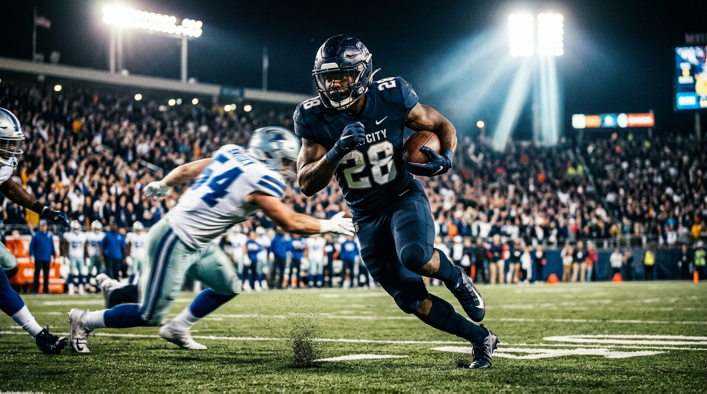
NFL running back rushing yards projections are my absolute bread and butter when it comes to breaking down a weekend slate. I blend film notes, team context, and AI simulations to turn all that weekly noise into clear ranges you can actually trust. If you bet props or set fantasy lineups, I will show you how to read medians, spots, and variance so you can act with real confidence instead of just crossing your fingers and hoping for the best.
Table Of Contents
What NFL running back rushing yards projections actually are
Data signals that actually move rushing yards projections
Building a transparent model that you can defend
Weekly workflow and QA that scales
A simple, transparent model spec you can copy
Interpreting results and taking action
Practical tools and templates to move faster
How to build, test, and iterate step by step
Where ATSwins fits and how to use model outputs
Common pitfalls to avoid
Quick examples of what changes what
Turning projections into card construction
A minimal calibration routine you can run weekly
A small glossary for clarity
Resource links you will use often
Final working notes you can copy each week
Conclusion
Frequently Asked Questions
What NFL running back rushing yards projections actually are
Rushing yards projections estimate how many yards a back will rack up on the ground in a specific matchup or across a full season. They are not fortune-telling predictions or random gut feelings. They are structured estimates that combine historical usage patterns, matchup context, and breaking news to build a complete distribution of likely outcomes.
Bettors rely on these distributions to price player props and same-game parlays, or to complement sides and totals when a team's game environment heavily leans toward the ground game. Fantasy managers use them to make tough start or sit calls, evaluate waiver wire priorities, and build daily fantasy lineups where median expectations and ceiling outcomes carry completely different strategic weights.
Understanding the difference between the median, ceiling, and floor is vital. The median represents the exact middle outcome where the back finishes above that mark half the time and below it the other half. This is the primary metric you compare against a sportsbook prop line. The ceiling sits around the upper edge of potential outcomes, which is perfect for tournament style fantasy contests or for hunting high-paying alternate over props when you spot positive environmental factors. The floor marks the lower range of realistic production, helping you identify safe cash game plays or fade overhyped, volatile market lines.
A single number completely hides the real story, whereas the shape of the full distribution tells you everything you need to know. Workhorse backs operating in run-first game scripts usually produce tight, predictable distributions. On the flip side, backfields split into complicated committees with unpredictable rotation patterns generate wide, chaotic distributions with low overall signal strength.
Uncertainty bands force serious accountability into your process. If your model outputs an outcome range between thirty-five and ninety-eight yards for a back and he finishes with sixteen, you immediately know you underweighted his downside usage or the negative game script. Bands help you fade fragile medians where soft usage assumptions create hidden risk. They also guide your bet sizing by giving you the green light to push higher confidence on narrow bands while demanding caution when ranges expand.
Data signals that actually move rushing yards projections
Every single projection model lives or dies based on the quality of its inputs. If you constantly chase superficial noise, you will end up rebuilding your setup every few weeks. Focus entirely on stable, interpretable signals that connect directly to expected attempts and efficiency.
Expected attempt volume is driven by lead back share, two-minute usage, and goal-line responsibilities. To measure a back's baseline role, look at recent rolling three to five game windows along with season-long expectations. Target snap rates, overall rush share, and first-down carry percentage rather than relying strictly on total snaps. If a running back gets yanked off the field whenever his team enters catch-up mode, his rushing ceiling takes a massive hit during trailing scripts. Goal-line carries carry immense value for touchdowns, but they also serve as a direct indicator of how much a coaching staff trusts a player, which naturally bleeds into regular early-down work.
Team rush rate over expectation measures how frequently a coaching staff chooses to run the ball relative to current down, distance, field position, time, and score. You should evaluate this metric using season-long data adjusted back toward the league average, blending it with coaching history and the quarterback's style of play. Apply this expected rush rate to projected neutral game plays to establish a firm baseline for overall team rushing volume.
Offensive line performance heavily dictates efficiency. Tracking yards before contact alongside gap and zone scheme success rates helps you map the specific fit between a running back and his blocking unit. Front five continuity and short-term injuries directly swing a team's efficiency on early downs. Weight yards before contact alongside independent offensive line grading, and adjust those numbers against the opponent's average defensive box counts to clear out structural bias.
Defensive schemes can act as run funnels. Certain defensive coordinators deliberately invite opposing offense to run the ball in order to take away explosive passing plays. These defenses often show high passing efficiency allowed while giving up average rushing numbers against lighter defensive fronts. Boost projected attempts slightly when a back faces a run-funnel defense, even if the team's projected trailing probability looks average on paper.
Pace and overall snap volume set the absolute capacity for production. More total plays directly translate into more possessions and potential rush attempts, provided the game script does not completely fall apart. Monitor seconds per snap in situation-adjusted environments alongside no-huddle rates to estimate total play volume for both sides of the ball.
Point spreads and game totals shape the script. Favored teams naturally run the ball far more often during the second half to bleed the clock. Heavy underdogs are forced to abandon the ground game and throw to keep up. High game totals increase overall play volume, which translates to extra late-game handoffs if the favored team establishes a comfortable lead. You should simulate game paths using the spread and total to roll up expected carry attempts based on script.
Injury reports require immediate adjustments across the entire depth chart. A questionable satellite back returning to action can instantly eat into a lead back's carry share. Injuries across the offensive line carry specific weight too, as missing tackles ruin outside zone plays and explosive potential, while missing guards or centers decimate yards before contact up the middle. Build distinct scenario splits for active versus inactive statuses, and execute your final updates ninety minutes before kickoff.
Weather thresholds can alter game plans dramatically. Sustained winds over fifteen miles per hour, heavy rain, or thick snow force teams to lean into the ground game. However, poor field conditions can simultaneously hurt footing and drag down efficiency per carry. Enclosed domes or retractable roofs completely eliminate atmospheric conditions, while cold temperatures alone rarely impact production. Always check stadium specific forecasts from official meteorology sources right before locking in your numbers.
Short-week travel schedules introduce subtle quirks. Thursday night games are notoriously sloppy, often featuring simplified game plans and a noticeable bump in conservative early-down runs. Long cross-country travel for early Sunday kickoffs can occasionally disrupt offensive rhythm, though it remains a minor variable compared to raw usage metrics.
Building a transparent model that you can defend
You want a projection model that you can clearly explain in under two minutes. Every single lever and adjustment must tie directly back to practical football logic.
Start by establishing rolling baselines for attempt volume and yards per carry. To calculate attempts, estimate total team plays by combining pace factors with league-average benchmarks adjusted for the specific matchup. Determine the team's overall run rate by layering their baseline average with their rush rate over expectation and script adjustments from the point spread. Allocate the primary back's share using a weighted blend of forty to fifty percent on the last three to five games, thirty to forty percent on season-long data, and ten to twenty percent on coaching priors. For efficiency baselines, start with the player's rolling two-year yards per carry, heavily regressed toward league averages. Layer on offensive line yards before contact and defensive box count expectations. Always cap extreme efficiency numbers, because yards per carry is inherently volatile.
Next, layer in opponent and offensive line adjustments. Adjust efficiency up or down based on the opposing defense's rushing metrics, weighting those adjustments by how often they face the run to strip out sample size noise. Modify efficiency figures using projected box counts and offensive line health. Apply subtle tweaks for home-field advantage or artificial turf versus natural grass surfaces, though these remain secondary factors. Multiplying your expected carry attempts by your adjusted efficiency gives you a clean initial rushing yards baseline.
Blend your historical priors with real-time weekly news using Bayesian updates or basic shrinkage methods. Set prior distributions for attempt volume and efficiency based on role stability and career variance. When news breaks regarding limited practice participation, beat writer notes about a hot-hand rotation, or an expected snap cap coming off an injury, update those distributions accordingly. Shrink individual metrics back toward team averages whenever a player is operating in a small sample size. This systematic process protects you from overreacting to single-game outliers.
Run at least five thousand simulations for every game environment. Model different game script paths based on the spread and total, tracking how game state changes across each quarter. For every individual simulation path, draw attempt totals from a conditional distribution tied to game script and role. Draw efficiency from your adjusted distribution, keeping a slight correlation between stacked box counts and offensive line health. Multiply attempts by efficiency to get total yards, capping extreme values at logical limits. Aggregate all simulation outputs to extract the median, floor, ceiling, and overall uncertainty intervals. Always build in a small, realistic probability for in-game injuries or benchings to keep the lower tail accurate.
Track your historical errors by specific categories to continuously recalibrate. Break your backtests down by point spread ranges, rush rate over expectation tiers, role stability types, offensive line health levels, and weather environments. Look closely for systemic bias. If you realize your model constantly overestimates carry volume for heavy underdogs, you need to reduce your script elasticity settings. If you consistently underestimate efficiency against light defensive boxes, increase your box count weighting. Document every single tweak in a running log and rerun your historical backtests to confirm improvement.
Weekly workflow and QA that scales
Establishing a rigid weekly rhythm prevents you from chasing random social media headlines and allows you to execute cleanly when Sunday arrives.
Early in the week, focus on ingesting baseline data. Process play-by-play data, pace metrics, rush rate over expectation, offensive line health, and player usage splits from reliable public databases like nflverse and Pro Football Reference. Refresh opponent efficiency metrics on rbsdm and pull defensive box counts alongside rushing yards over expected from NFL Next Gen Stats. This step generates your initial medians with wide, unrefined uncertainty bands.
Midweek is all about parsing news and evaluating player splits. Dig through official practice reports and categorize target players as full, limited, or non-participants. Re-evaluate specific role assignments including two-minute drill work, pass-protection trust, and goal-line preferences. Make modest updates to your baseline shares, but never let a single coach quote completely overturn a well-established usage trend. This results in your version two medians with refined variance settings.
By Friday, turn your attention to weather forecasts and final offensive line injury designations. Pull precise stadium forecasts from the National Weather Service, flagging games with winds expected to top fifteen miles per hour or significant precipitation. Confirm offensive line starting lineups and identify confirmed inactives. This yields your version three projections, complete with weather adjustments and contingency splits for questionable players.
Saturday night is reserved for executing your primary simulation runs. Execute five to ten thousand simulation passes per game, saving the final medians alongside your eighty and ninety percent confidence intervals. Flag fragile medians that feature wide distributions so you know where caution is required. Publish these structured outputs directly to your primary tracking sheet.
Sunday morning requires a quick, focused refresh. Incorporate official inactive lists ninety minutes prior to kickoff, rerunning simulations for any game impacted by late scratches. Send out immediate alerts for sudden role shifts, producing your final timestamped projection set right before games begin.
Your ongoing responsibility involves backtesting and running diagnostic reviews. Track weekly errors across different team archetypes and play styles. Identify the primary drivers behind major misses, whether you underweighted a sudden usage shift, missed an in-game injury tail risk, or got burned by garbage-time rushing volume. Log these findings in a persistent changelog, updating model weights only after accumulating multi-week evidence.
Running through a simple quality assurance checklist keeps your output clean. Verify that team carry projections align with the spread and overall rush rate. Ensure individual running back shares match practice tracking and coaching patterns. Confirm efficiency figures accurately account for line health and defensive match-ups. Double-check wind and rain inputs for outdoor venues, and make sure your uncertainty bands remain realistic rather than artificially narrow. Finally, verify that your calculated medians sit comfortably within historical expectations for the player's scheme.
A simple, transparent model spec you can copy
You can build a fully functional model using a clean set of core inputs. Gather team-level plays based on pace and matchup, team run rates driven by script and rush rate over expectation, individual attempt shares based on situational roles, and regressed baseline efficiency figures. Layer on efficiency tweaks for offensive line health, box counts, and defensive matchup ratings, followed by minor modifiers for practice news, weather, and venue surfaces.
Model attempt volumes using a truncated normal distribution set to zero or higher. Model efficiency using a lognormal or truncated normal distribution, enforcing a hard floor near two yards per carry and a reasonable cap near seven and a half yards per carry to control extreme mathematical tails.
Execute your simulation by branching game scripts using the point spread and total, drawing attempts conditional on how those script branches unfold. Multiply attempts by efficiency to calculate total rushing yards, then aggregate those results into P15 floors, P50 medians, and P80 ceilings. Output these metrics alongside a visual stability tag and sensitivity indicators for offensive line scratches, wind shifts, or backup player inactives.
Keep operational notes structured cleanly for every player you analyze. Log the player's name, team, baseline attempts, lead share, and total team rush volume. Record baseline efficiency alongside adjusted efficiency, weather conditions, and missing offensive line starters. Save the final median, floor, and ceiling outputs alongside specific risk flags or role notes. This structure maintains total transparency across your weekly process.
Interpreting results and taking action
Translating raw probability distributions into actionable betting edges requires real discipline.
Always fade fragile medians that feature unusually wide output bands. If a player's calculated floor to ceiling range spans all the way from forty to one hundred and ten yards, a median of sixty-eight is fundamentally fragile. That wide spread indicates a messy committee split or a volatile role. You should drastically reduce your stake size or pass entirely unless the line is severely out of whack. Conversely, if a back's floor to ceiling range sits between sixty-two and ninety-five yards with a median of seventy-eight, his volume is remarkably stable, making him a much stronger candidate for a prop wager at fair market odds.
Look to stack correlated edges whenever possible. Running back carry overs naturally pair well with favored teams playing in windy weather, run-heavy offenses operating behind healthy offensive lines, or defenses that invite the run by dropping coverage. Avoid taking opposing positions that fight against core game correlations, such as betting a back's carry over while taking the opposing team on the point spread, unless you are targeting a very specific game flow scenario.
Adjust quickly for major market movements and late inactive reports. If sportsbooks steam a favorite from minus two up to minus four and a half, the expected game script just became noticeably more run-heavy, requiring an immediate recalculation of attempt volume. If a pass-catching backup is ruled out, the primary back might absorb additional two-minute snaps, raising his floor and boosting total carries. If a star left tackle is scratched close to kickoff, dock the back's efficiency moderately, particularly on outside running concepts. Establish firm thresholds for re-betting, such as requiring a multi-point spread move or a major role change before altering your existing positions.
When sharing analysis with clients or colleagues, communicate clear ranges rather than isolated numbers. Frame outputs with context like stable volume with efficiency risk, or fragile usage with high script dependency. When comparing your ranges against multiple books, use your floor and ceiling thresholds to guide your leans. If your calculated floor sits higher than a published sportsbook line, the over carries strong appeal. If your calculated ceiling falls below a posted total, the under becomes the preferred angle.
Consider a practical example featuring a lead back as a modest home favorite. The team is favored by three and a half points with a total of forty-two, holding a positive rush rate over expectation, a slow pace, and a fully healthy offensive line. The opposing defense boasts strong pass coverage but weak run defense, while weather conditions show light ten mile per hour winds. The model projects modest overall play volume with an elevated run rate. The lead back commands a seventy-two percent share of rushes in neutral and positive scripts, holding an adjusted efficiency of four point four yards per carry. This generates an expected median of eighteen point five carries and eighty-one rushing yards, with a tight distribution ranging from sixty to one hundred two yards. This represents a prime candidate for an over wager if sportsbooks list the line in the mid-seventies.
Now contrast that with a committee back playing on the road as a significant underdog in poor weather. The team is a six and a half point underdog with a low thirty-eight total, a negative rush rate over expectation, a missing starting left tackle, and facing twenty mile per hour winds with rain. While wind generally encourages running, the trailing game script reduces total carries for a back who loses work during two-minute situations. His share sits in an uncertain fifty to fifty-eight percent range, while his efficiency drops to three point seven yards per carry due to line injuries and a tough matchup. This produces an expected median of just twelve carries for forty-four yards, wrapped in a wide distribution spanning from twenty-five to sixty-seven yards. This fragile median signals a clear pass or a lean toward the under if the market line is inflated.
Size your wagers according to uncertainty levels. Allocate larger stakes when you spot narrow intervals, strong matchup alignment, and multiple converging signals like high rush rates, healthy blocking, favorable spreads, and wind. Scale down to smaller stakes when ranges widen or signals conflict, such as an underdog back playing in high wind with an uncertain committee split. Pass on the game entirely if you find yourself relying on unverified practice rumors, if the market has already swallowed the value, or if high uncertainty cancels out the price edge.
When news breaks, issue rapid updates with clear timestamps. A backup running back scratch can instantly add three to five carries to the starter in positive scripts. An offensive line injury typically docks efficiency by two-tenths to three-tenths of a yard per carry. A three-point spread adjustment shifts carry totals by one and a half to two attempts depending on direction. Keeping your updates transparent ensures everyone understands exactly what changed and why.
Practical tools and templates to move faster
Streamlining your workflow requires automating your data pipelines. Use nflverse to automatically pull play-by-play data, updated rosters, and game results. Pull offensive and defensive efficiency metrics from rbsdm on a scheduled weekly cache. Track offensive line continuity and injury statuses manually or via scraped reports, and pull box counts and rushing yards over expected from NFL Next Gen Stats. Always rely on official National Weather Service forecasts for stadium weather metrics, and maintain a strict changelog to track all model revisions over time.
Organize your weekly workbench across dedicated spreadsheet tabs. Dedicate the first tab to team-level baselines like pace, script, and spread totals. Use the second tab for running back role tracking, including situational carry shares and specialized snap rates. Place efficiency baselines, line health, box counts, and defensive ratings on the third tab. Use the fourth tab to log news modifiers and subjective adjustment weights, and reserve the final tab for simulation outputs featuring medians, ranges, and stability tags.
How to build, test, and iterate step by step
Building a durable projection system requires following a methodical, iterative path.
Start by defining your underlying units and baseline priors. Choose rolling time frames, such as a five-game window for role usage and a two-year window for efficiency metrics, applying consistent regression weights back toward league averages. Next, construct team-level play projections by estimating total snaps and applying run-pass splits derived from script and rush rate over expectation. Always double-check these numbers against season averages to prevent unrealistic outputs.
Allocate carry attempts across the depth chart based on situational roles. Assign specific shares for neutral game flows, trailing two-minute scripts, and positive closing environments. Document special exceptions, such as pass-protection issues for rookies or coach comments regarding a hot hand, applying small, controlled weights to account for them.
Adjust efficiency metrics starting from the player's regressed yards per carry baseline. Layer on modifications for offensive line health, defensive box count expectations, and opponent efficiency metrics. Add minor tweaks for venue surface and home-field factors where appropriate.
Execute your simulation suite using at least five thousand iterations per matchup, incorporating branching game scripts to reflect changing field conditions. Save calculated medians alongside your eighty and ninety percent uncertainty bands.
Validate your weekly outputs by comparing calculated medians against closing sportsbook prop lines. Finding huge discrepancies between your model and the market usually points to an input error or an unmodeled usage shift rather than an instant betting edge. Track your absolute errors and evaluate your overall calibration to confirm whether eighty percent of real-world results actually fall inside your calculated eighty percent confidence intervals.
Recalibrate your setup by specific categories over time. Adjust your variance settings if you discover you are miscalibrated on committee backfields, heavy underdogs, or teams dealing with offensive line injuries. Only update primary model coefficients after gathering multi-week evidence across a solid sample size.
Operationalize your final workflow by building a strict Sunday morning checklist. Prepare contingency scenario splits for all questionable players, and ensure every published projection set includes an immutable timestamp.
Where ATSwins fits and how to use model outputs
ATSwins is an AI-powered sports prediction platform built to synthesize complex data signals quickly and present actionable ranges rather than just a single, isolated number. It offers data-driven picks, player props, betting splits, and profit tracking across the NFL, NBA, MLB, NHL, and NCAA.
When combining your personal modeling efforts with platform metrics, use ATSwins distributions to validate or challenge your calculated medians. If ATSwins displays a noticeably wider output range on a specific player, dig deeper into the matchup. It often signals elevated role uncertainty or hidden offensive line concerns that your manual inputs may have underweighted. When multiple distinct models align, such as your calculated median and the ATSwins projection both sitting well above the published market line with tight confidence bands, you have a prime scenario to execute a confident wager while maintaining proper bankroll management. Furthermore, leverage ATSwins automated tracking to monitor late-breaking weather shifts and official inactive reports before placing your final Sunday wagers.
Common pitfalls to avoid
Overfitting to single-game samples is easily the most common trap in player projection work. A backup running back breaking off twenty-five carries in a blowout win does not instantly rewrite a season-long committee structure.
Ignoring defensive box counts will constantly throw off your efficiency numbers. A running back facing an eight-man box on sixty percent of his snaps operates in a completely different physical environment than one facing light seven-man boxes all afternoon.
Forgetting that carry volume and efficiency interact dynamically leads to flawed outputs. Carry attempts and yards per carry are not independent variables; game script directly impacts both metrics simultaneously as defenses adjust their alignment to the clock and score.
Misinterpreting coach quotes will introduce unnecessary noise into your model. Take media comments with a grain of salt, assigning small weights to verbal reports until you see concrete on-field usage confirm the shift.
Skipping extreme value controls produces chaotic simulation tails. You must place reasonable caps on yards per carry distributions and build in a non-zero probability for in-game injuries or unexpected benchings to keep your lower tail realistic.
Overreacting to basic weather descriptions leads to bad bets. High winds disrupt passing games and force rush attempts, whereas cold temperatures alone have virtually zero predictive impact on game plans. Domes and retractable roofs completely neutralize atmospheric factors, so never dock a team's efficiency based on cold weather if they are playing indoors.
Quick examples of what changes what
When a primary backup running back is ruled inactive, expected carry volume for the starter typically jumps by two to five attempts depending on the backup's usual script role. Efficiency remains largely neutral, unless the backup served as the dedicated short-yardage hammer, in which case the starter's yards per carry might see a slight bump due to taking on more open-field snaps.
When a point spread shifts from minus one to minus four, expected carry volume for the favored lead back increases by one to two attempts as late-game closing scripts become far more likely. Efficiency can see a minor positive bump if the opposing defense drops extra defensive backs to guard against play-action passing.
When a starting left tackle is scratched right before kickoff, efficiency drops by two-tenths to three-tenths of a yard per carry, with the impact hitting hardest for teams that rely heavily on outside-zone running concepts. Carry attempts may also drift downward slightly if the loss in pass protection leads to more stalled drives and negative game scripts.
Turning projections into card construction
Start your weekly betting routine by pre-shopping lines across multiple sportsbooks. Look for a minimum edge threshold of five to eight yards between your calculated median and the published market line, requiring smaller gaps when dealing with tight, stable output bands.
When exploring alternate prop lines, look at your P85 ceiling outputs for ladder wagers when multiple positive volume signals align. Pair your picks intelligently by combining running back carry overs with team moneyline wagers in run-positive scripts, or taking running back rushing unders when an underdog faces a tough run defense that commands stacked boxes.
Timing your bets properly is essential for capturing market value. Early in the week, focus on attacking mispriced opening spreads that will shift game script projections as the market settles. Late in the week, pivot your focus toward exploiting role clarity and weather updates after official inactive reports drop.
A minimal calibration routine you can run weekly
Check your total coverage metrics every single week. Exactly eighty percent of real-world player results should land within your calculated eighty percent uncertainty intervals. If your backtests show only sixty-five percent of outcomes landing inside your band, your model is operating too tight and requires wider variance settings.
Check for systemic prediction bias by evaluating mean error across specific sub-categories. If your calculated error diverges significantly from zero within specific spread ranges or offensive line health tiers, adjust your underlying weights accordingly.
Track market drift to evaluate your baseline script inputs. If your calculated medians systematically lag behind final closing lines, introduce market-derived script priors as a soft input to keep your baseline aligned with sharp market movement.
A small glossary for clarity
Expected Points Added measures the true value of an individual play in terms of points relative to down, distance, and field position.
Success rate defines the percentage of plays that yield positive Expected Points Added, keeping an offense on schedule.
Rush rate over expectation tracks how frequently a team chooses to execute a run play compared to league-wide expectations given the exact game state.
Box count represents the total number of defensive players lined up in close proximity to the line of scrimmage at the snap.
Yards before contact measures the exact distance a running back travels past the line of scrimmage before meeting the first defender.
Resource links you will use often
For detailed box counts and rushing yards over expected metrics, consult NFL Next Gen Stats.
For team-level efficiency, play-by-play breakdown, and defensive ratings, utilize rbsdm.
For historical game logs, situational splits, and target shares, search Pro Football Reference.
For open-source play-by-play databases and roster tracking, access nflverse.
For venue weather forecasts and wind reports, check the National Weather Service.
For advanced sports predictions, betting splits, and model ranges, visit ATSwins.
Final working notes you can copy each week
Keep a clean text template handy to log your weekly analysis for every game slate.
Team context Spread and total: Situation-adjusted pace: Season and regressed rush rate over expectation:
Role splits Lead back rush share across neutral, positive, and negative scripts: Two-minute drill role: Goal-line assignment:
Efficiency metrics Regressed player efficiency baseline: Missing offensive line starters: Baseline yards before contact: Opponent defensive efficiency ratings: Defensive box count tendencies:
Environmental factors Venue and roof status: Sustained wind speed: Precipitation type and intensity:
Simulation outputs Median carry attempts: Adjusted yards per carry: Rushing yards distribution across floor, median, and ceiling: Assigned stability tag:
Change log Midweek updates and notes: Inactive report impacts: Late market movement:
Using this operational structure maintains complete transparency, keeps your process fast, protects you from overreacting to surface noise, and helps you make consistent, data-driven decisions for sports betting and fantasy football.
Conclusion
Projecting NFL running back rushing yards successfully requires working with structured probability ranges rather than anchoring to a single prediction. Focus on expected volume, game script dynamics, and weather factors, then continuously validate and refine your outputs. Track subtle role changes, blend historical priors with fresh news, and respect the natural uncertainty inherent in every game slate. If you want to elevate your weekly preparation, ATSwins provides an AI platform with data-driven picks, player props, betting splits, and profit tracking across the NFL, NBA, MLB, NHL, and NCAA, offering free and paid options to help you make smarter decisions.
Frequently Asked Questions
What are NFL running back rushing yards projections, really?
NFL running back rushing yards projections are structured mathematical estimates of how many yards a back will gain in a specific matchup or season. They are built by blending usage metrics like carry shares and snap rates with team tendencies, offensive line health, and defensive matchups, then simulating those variables thousands of times. High-quality projections provide a median expectation alongside a range of outcomes to account for variance.
Which factors move NFL running back rushing yards projections the most?
Expected carry volume is the single largest factor, driven by lead back share, goal-line usage, and overall team rush rate over expectation. The point spread and game total dictate expected game scripts, while weather conditions like high winds or heavy rain can push teams toward more run attempts while impacting efficiency per carry. Late injuries across the running back room or offensive line alter projections immediately.
How should I use NFL running back rushing yards projections for props and fantasy?
Use projections as ranges rather than absolute numbers. Compare calculated medians against posted sportsbook prop lines to find structural edges for wagers. Ceilings help you target high-upside daily fantasy plays or alternate over props, while floors indicate safe cash game options. In seasonal fantasy, use ranges to navigate start or sit decisions, adjusting your lineups on Sunday morning based on weather and active lists.
Do weather, injuries, and game script change projections late in the week?
Late updates drastically alter model outputs. An inactive backup running back concentrates carry share onto the starter, while a scratch along the offensive line docks yards before contact. Sustained winds over fifteen miles per hour increase carry volume while slightly dampening overall efficiency. Re-run your simulation models as soon as major news breaks and do a final refresh once official inactive lists drop prior to kickoff.
How does ATSwins help with NFL running back rushing yards projections?
ATSwins leverages AI modeling to deliver data-driven picks, player props, betting splits, and bankroll tracking across major sports leagues. The platform provides projection ranges complete with calculated medians and confidence bands, incorporating pace factors, offensive line grades, and weather reports. This allows you to spot gaps between model outputs and published sportsbook lines while receiving alerts on key updates before market prices adjust.