

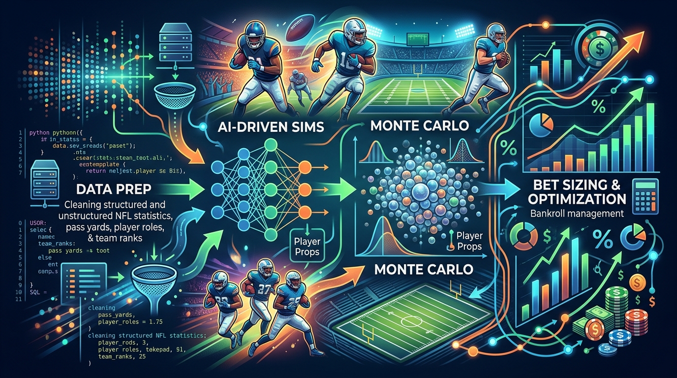
Building an NFL player prop simulation model sounds complicated at first. There are player stats, team tendencies, injuries, weather, coaching decisions, game script, market movement, and plenty of uncertainty packed into a single player prop.
But the basic idea is simple. You are trying to estimate how often a player reaches a specific statistical outcome under the conditions of an upcoming game. From there, the goal is to turn those probabilities into fair prices, compare them with available betting lines, and determine whether the difference is meaningful.
At ATSwins, this process starts with opportunity rather than just averages. A receiver averaging 62 yards per game does not automatically have a 50% chance of going over 62. His routes, targets, team pass volume, matchup, injuries, weather, and expected game script all matter.
That is why simulation is useful. Instead of producing one projection, the model can run thousands of possible versions of the game. Some scenarios have more plays, some have fewer. A receiver can see eight targets in one trial and 12 in another. A running back can receive 18 carries in a positive script and 11 when his team falls behind.
After thousands of trials, the model can estimate how often a player clears a betting line. The result is a full probability distribution that can support fair pricing, risk management, and better decision making.
Table of Contents
Problem Framing and Data Intake
Modeling Approach and Feature Engineering
Simulation and Calibration
Edge Sizing and Operations
Practical Step-by-Step: From Raw Data to an Actionable Pick
How ATSwins Fits Into the Process
Implementation Tips That Save Time
Common Pitfalls and How to Avoid Them
Quick Recipes for Popular NFL Player Prop Markets
QA and Model Monitoring
Scaling to Same-Game Combos
Roadmap for Improving the Model
Conclusion
Frequently Asked Questions
Problem Framing and Data Intake
Start With Tradable Markets
The first step is defining exactly what the model should predict. NFL player props can cover passing, rushing, receiving, touchdowns, attempts, receptions, targets, and combination markets. Each market has different statistical behavior, so every prop should be modeled according to the events that create it.
Passing yards depend heavily on team dropbacks, quarterback efficiency, pressure, completion depth, and game script. Receiving yards depend on routes, targets, catch probability, air yards, yards after the catch, and opportunity. Rushing yards depend on attempts, offensive line performance, game state, and yards per carry.
Touchdown props are different because touchdowns are relatively rare and naturally volatile. The model needs to recognize that one play can completely change the result.
Connect Each Prop to Real Inputs
A clean model makes every market traceable to measurable inputs. Receiving yards can be connected to targets, catch probability, average depth of target, and yards after the catch. Receptions can be connected to targets and catch rate. Targets can be connected to routes and targets per route. Routes can be connected to team dropbacks and route participation.
Rushing attempts can be connected to team rushing plays and player rush share. Rushing yards can then be modeled from attempts and expected yards per carry. Touchdowns can be connected to red-zone opportunities, goal-line usage, target share, carry share, and conversion probability.
This structure makes projections easier to audit. If a receiving projection suddenly rises, the model should show whether the change came from more routes, more targets, higher team volume, a better matchup, or another input.
Build a Reliable Data Pipeline
Good simulations depend on good inputs. Historical play-by-play data provides information about offensive plays, pass attempts, rushing attempts, touchdowns, field position, and game state. Player usage data adds information about snaps, routes, targets, and carries.
The model should also account for team tendencies, opponent tendencies, injuries, expected player roles, weather, rest, travel, and market lines. Every update should be timestamped so historical tests use information that was actually available before each game.
Player and team identifiers should also be standardized. Different data feeds can use different naming conventions, and a bad join can quietly create missing or duplicated statistics.
Market lines should be stored with their price, source, market name, and timestamp. This allows the model to compare its fair price with the number that was actually available.
Handle Injuries and Partial Games
Injuries are especially important because an injury changes more than one player. If a starting receiver leaves, his routes and targets must be redistributed. Another receiver, tight end, or running back can gain opportunities.
The simulation should therefore create multiple workload scenarios. A player might play his normal role in most trials, see reduced usage in others, or leave early in a smaller group of trials.
The same logic works for snap caps and uncertain roles. Instead of forcing an exact workload, the model should carry uncertainty through every trial.
Modeling Approach and Feature Engineering
Start With Usage
For NFL player props, usage is often more important than raw talent. A talented receiver cannot produce a huge receiving total without enough routes and targets. A strong running back needs enough carries to reach a rushing line.
Projected snap share, route participation, target rate, rush share, and red-zone involvement should therefore sit near the center of the model.
Recent usage deserves attention, but it should not completely replace longer-term information. A player can have a huge role for two games because of an injury and then return to a smaller role once the roster changes.
Team Pace and Play Volume
Player props are connected to team volume. A fast offense can create more opportunities, while a slower offense can reduce them. Expected pace should therefore be modeled rather than copied directly from a season average.
Pass rate matters just as much. More passing plays create opportunities for quarterbacks and receivers, while fewer passing plays can reduce their ceilings. At the same time, rushing opportunities can increase.
The model should simulate these tradeoffs instead of projecting each player independently.
Game Script and Matchup
Game script can change offensive behavior throughout a game. A favorite protecting a lead may run more often late, while an underdog chasing points can increase its passing volume.
The spread and total can provide useful context for the expected environment, but they should not be treated as perfect predictions.
Defensive matchup factors can also influence props. Pressure can encourage quicker throws and affect depth of target. Coverage tendencies can influence where targets are distributed. Strong run defense can encourage passing.
These variables should usually create measured adjustments rather than enormous swings.
The spread and total can provide useful context for the expected environment, but they should not be treated as perfect predictions.
Bayesian Shrinkage
Small samples create noise. A receiver with a 35% target share over two games may not truly have a 35% role. Bayesian shrinkage helps combine recent observations with longer-term expectations.
The same idea can be applied to catch rate, yards after the catch, yards per carry, red-zone usage, and other player rates.
Recent information should move the projection when the role genuinely changes, but extreme short-term results should be pulled toward more stable priors.
Outcome Distributions
Different statistics need different distributions. Counts such as targets, receptions, and carries can use Poisson or negative-binomial approaches when overdispersion exists. Receptions can also use a beta-binomial structure because catch probability itself has uncertainty.
Yardage often has a longer right tail, so lognormal or gamma-style distributions can be useful. Touchdowns can be modeled through Bernoulli or Poisson-binomial approaches based on opportunities.
The goal is not to pick a distribution because it sounds sophisticated. The goal is to choose a structure that resembles the actual behavior of the statistic.
Correlation Between Players
Props are not independent. Receivers on the same team share quarterback attempts. Running backs and quarterbacks share rushing opportunities. Team pace affects almost everyone.
The simulation can use shared latent variables for pace, pass rate, weather, and game state. If the team throws more than expected in a trial, multiple receivers can benefit together.
Target allocation can also be modeled jointly. A Dirichlet-multinomial approach can allow target shares to vary while still respecting the team's total passing volume.
Simulation and Calibration
Monte Carlo Simulation
Once the inputs are ready, the model can run thousands of game trials. A practical simulation can use 10,000 or more trials.
Each trial starts by generating the team environment, including expected plays, pace, pass rate, rushing rate, and game state. Next, player participation is drawn. Routes, snaps, targets, and carries are then allocated according to projected roles.
For receivers, targets become catches and receiving yards. For rushers, attempts become rushing yards. Red-zone opportunities become touchdown chances.
At the end of every trial, the model stores the player's final statistics. After thousands of trials, the model has a distribution that can answer questions about standard lines, alternative lines, ladders, and combinations.
Propagating Uncertainty
One of the most useful parts of simulation is carrying uncertainty through the entire process. If snap expectations are uncertain, that uncertainty should affect routes. Route uncertainty should affect targets. Target uncertainty should affect receptions and yards.
This is much more realistic than projecting 75% snaps, 8 targets, and 62 yards as fixed numbers.
Role-change scenarios should also be included. If one receiver is limited, another player's route share can increase. If a running back loses passing-down work, another player can receive those opportunities.
Calibration and Backtesting
A model can produce impressive projections while still being poorly calibrated. Calibration means predicted probabilities should match actual frequencies over time.
If the model assigns a 60% probability to an outcome, that outcome should happen close to 60% of the time across a large sample.
Brier score is useful for binary outcomes such as touchdown markets. CRPS is useful for continuous statistics such as receiving or rushing yards. Predictive interval coverage can also show whether the model is too confident or too conservative.
Backtesting should be time aware. Train on earlier games and test on later games so the process resembles real forecasting. Historical tests should use only information available before the game.
Monitoring Model Drift
NFL teams change during the season. Players return from injury, coaching strategies shift, quarterbacks develop new tendencies, and depth charts change.
For that reason, calibration should be monitored continuously. If performance deteriorates, investigate whether the problem is player usage, team volume, efficiency, injury assumptions, or another feature.
Edge Sizing and Operations
Convert Simulation Results Into Prices
After simulation, calculate the percentage of trials in which a player goes over or under the posted line.
That probability becomes the model's estimate for the outcome. It can then be converted into a fair price and compared with the market price.
The difference represents potential value, not a guarantee. A model probability is still an estimate, and uncertainty remains.
Price matters just as much as the projection. A favorable statistical expectation can become a poor bet if the market price is too expensive.
Alternative Lines and Ladders
A full distribution makes alternative lines much easier to evaluate. Instead of building a separate model for every receiving yardage line, one simulation can estimate the probability of clearing many different thresholds.
The same applies to receptions, rushing yards, passing yards, and attempts.
This helps identify where the price becomes attractive and where the market has gone too far.
Staking and Risk
Even a strong model will have losing streaks. Stake sizing should therefore reflect both estimated edge and uncertainty.
Fractional Kelly can provide a framework for sizing positions while reducing the volatility associated with full Kelly. High-variance markets such as longest reception and anytime touchdowns generally deserve more conservative exposure than narrower count markets.
Correlation also matters. Several receiver overs from the same team can create much more risk than the individual stakes suggest because they depend on the same passing environment.
Practical Step-by-Step: From Raw Data to an Actionable Pick
Prepare the Data
Start with several seasons of historical information and combine it with current-season data. Calculate rolling usage rates, load current injury information, estimate expected roles, account for weather, and collect current market lines.
Build the Features
Create team features such as pace, pass rate, offensive efficiency, and expected game script. Create player features such as snap share, route participation, target rate, rush share, catch rate, and red-zone usage.
Then add opponent and environmental factors.
Update the Priors
Use recent performance to update longer-term expectations. Apply shrinkage so a small sample does not completely change the projection.
Run the Simulation
Run at least 10,000 trials when practical. Include uncertainty around pace, pass rate, snaps, routes, targets, carries, efficiency, weather, and game state.
Keep correlated variables connected.
Price the Market
Calculate over and under probabilities for each available line. Convert them into fair prices and compare them with the market.
Explain the Pick
A useful recommendation should have a clear reason. The driver might be increased route participation, higher expected passing volume, a matchup adjustment, or an injury creating additional opportunities.
The explanation should connect directly to the model.
Monitor the Pick
Late injury news or major market movement can invalidate an earlier projection. Re-simulate when meaningful information changes.
After the game, save the result and compare it with the predicted distribution.
How ATSwins Fits Into the Process
ATSwins brings data-driven sports analysis into a practical prediction workflow. The platform provides AI-powered sports predictions, player props, betting splits, and profit tracking across NFL, NBA, MLB, NHL, and NCAA markets.
For NFL player props, a simulation-based process can combine player usage, team environment, matchup information, injuries, and market prices. The goal is to turn those inputs into probabilities and fair prices that are easier to understand.
Transparency matters here. A pick should have a reason behind it, and the model should update when the underlying situation changes.
Profit tracking also provides a useful way to review whether the model is producing sustainable results instead of focusing only on short-term wins and losses.
Common Pitfalls and How to Avoid Them
Double-counting team opportunities is a major problem. If a quarterback is projected for 38 attempts, receiver targets cannot add up to an impossible number.
Overreacting to one game is another issue. A huge performance can reflect matchup, game script, injuries, or randomness rather than a permanent skill change.
Ignoring correlation can make teammate and same-game probabilities unrealistic.
Unit confusion can also create errors. Make sure every variable has a clear definition and unit.
Weather should be handled carefully. Strong wind can matter significantly, while light rain may have a much smaller effect.
Finally, check whether projections make sense together. If team pass volume falls, it should be difficult for every receiver to simultaneously receive a major projection increase.
Quick Recipes for Popular NFL Player Prop Markets
Receptions
Estimate team dropbacks, then projected routes. Use targets per route to estimate opportunities and a probability distribution to model catches.
Once the reception distribution exists, use it to price standard lines and alternative lines.
Receiving Yards
Start with projected receptions and expected yards per catch. Average depth of target, yards after the catch, route role, and matchup can influence the distribution.
Allow for occasional explosive outcomes rather than forcing everything into a simple normal distribution.
Rushing Yards
Project team rushing volume and player rush share first. Then model attempts and yards per carry.
Game script, goal-line work, offensive line conditions, and quarterback rushing can all influence the final distribution.
Touchdowns
Estimate red-zone opportunities and then allocate them among players. Goal-line carries and red-zone targets should influence touchdown probabilities.
Because touchdowns are volatile, avoid excessive confidence.
Scaling to Same-Game Combos
A strong simulation can estimate joint probabilities for same-game combinations.
If two receivers are both projected to go over their reception lines, their joint probability is not necessarily the product of their individual probabilities. They share the same quarterback and team passing environment.
The simulation already contains those shared variables, so the joint result can be calculated directly from the trials.
This approach can also evaluate quarterback passing yards with receiver receiving yards or running-back rushing volume with team scoring.
The main caution is exposure. Several highly correlated positions can create a concentrated risk profile.
Conclusion
Building an NFL player prop simulation model is about breaking a complicated game into measurable pieces.
Start with team volume. Estimate player roles. Project snaps, routes, targets, carries, efficiency, and red-zone opportunities. Then connect those inputs through a simulation that respects uncertainty and correlation.
The biggest advantage of this approach is that it produces a distribution instead of one number. That distribution can be used to estimate probabilities for standard lines, alternative lines, ladders, and combinations.
Calibration is just as important as prediction. A model needs to know when it is uncertain and must be tested against future games rather than only historical examples that make it look good.
ATSwins uses a data-driven approach to sports prediction, player props, betting splits, and profit tracking across NFL, NBA, MLB, NHL, and NCAA markets. The broader goal is to make sports analysis more structured, transparent, and useful.
There is no perfect NFL player prop model. The goal is to build a system that learns from new information, respects uncertainty, explains its decisions, and separates meaningful edges from projections that only look impressive.
Frequently Asked Questions
What is an NFL player prop simulation model?
An NFL player prop simulation model uses player statistics, team trends, injuries, matchups, game script, and other factors to simulate thousands of possible game outcomes and estimate the probability of a player going over or under a betting line.
How accurate are NFL player prop simulations?
No simulation can guarantee a winning result. However, using large amounts of historical data, realistic player usage, game conditions, and proper calibration can help produce more reliable probability estimates.
What factors affect NFL player prop predictions?
Important factors include player snaps, routes, targets, carries, team play volume, pass rate, game script, injuries, opponent matchup, weather, and expected player role.
Can simulations help find value in NFL player props?
Yes. A simulation can compare its estimated probability with the probability implied by the betting market. When there is a meaningful difference, it may indicate a potential betting edge.
How does ATSwins help with NFL player props?
ATSwins uses data-driven sports analysis to evaluate player props, predictions, betting splits, and other factors across major sports, helping users make more structured and informed betting decisions.