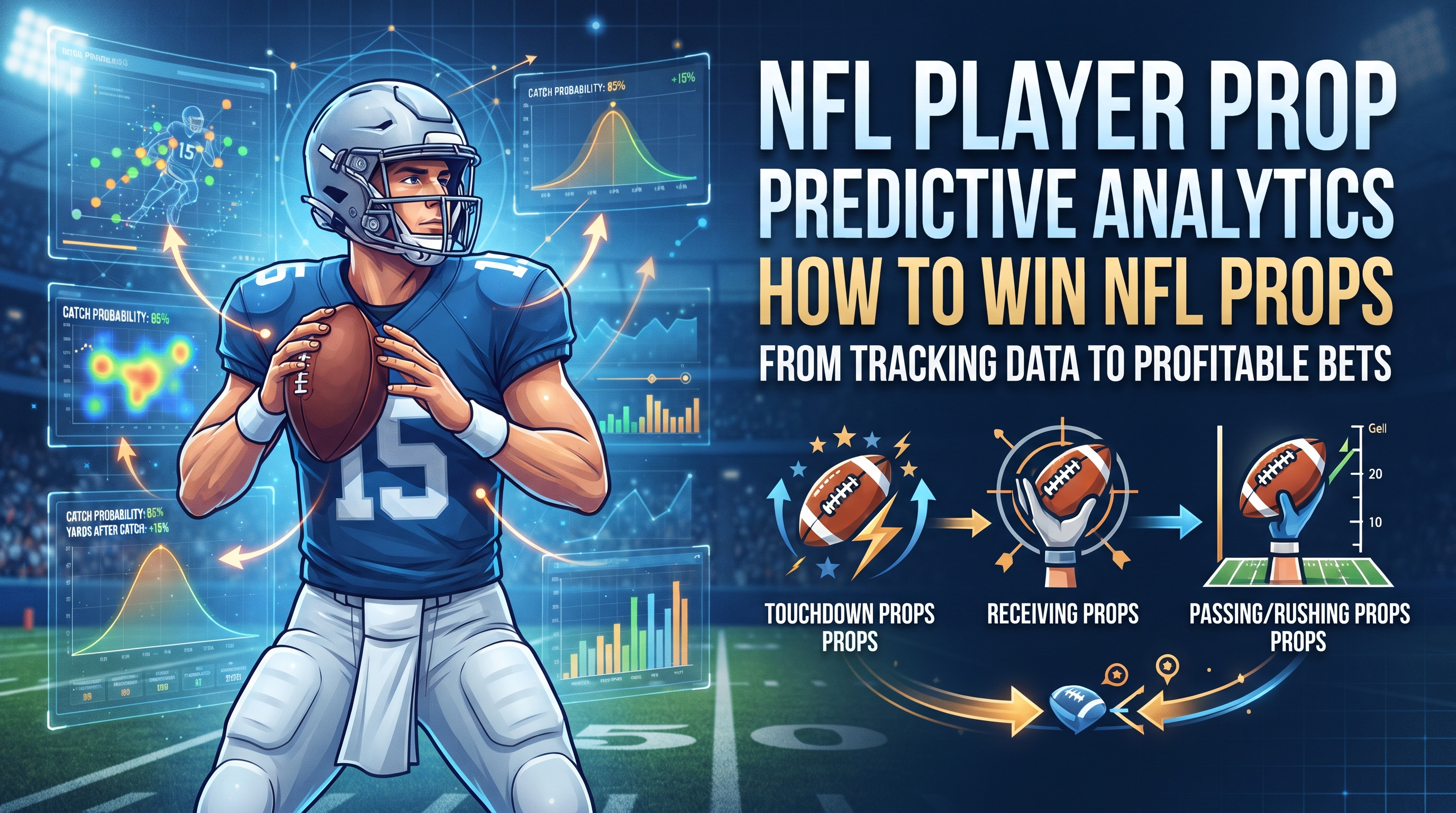
Player props don’t have to feel like a coin flip. I’ll show you how I use NFL tracking data, context, and AI models to turn receptions, yards, and touchdowns into clean probabilities and fair prices. We’ll keep it practical—what to pull, how to model it, and when to bet—so you can spot true edges. 

Building Predictive Edges for NFL Player Props: From Tracking Data to Prices

Problem framing for NFL player prop predictive analytics

What player props are (and why they behave differently from sides/totals)

Player props are wagers on individual player outcomes rather than team results. Books offer a wide set of markets for skill players and quarterbacks, often including passing metrics like attempts, completions, yards, touchdowns, and interceptions, alongside rushing measures such as attempts, yards, touchdowns, and long rushes. Furthermore, receiving markets cover targets, receptions, yards, touchdowns, and long receptions, while combo bets merge rushing and receiving yards, pass-rush-rec yards for quarterbacks, or occasionally receptions and rush attempts. Specials round out the selection with first or anytime touchdowns, alternate lines, and ladder markets.

Props move on information and usage signals much faster than traditional sides or totals. They are exceptionally sensitive to a team’s strategic game plan, unforeseen injuries, direct matchups, and evolving game scripts. That dynamic creates both the underlying opportunity and the inherent risk.

Predictive vs descriptive modeling

Descriptive models explain what happened by summarizing prior games, historical hit rates, efficiency statistics, and basic averages. In contrast, predictive models forecast what is likely to happen next by using current contextual variables. These variables include a player's skill set and projected role for today, such as snap share and route participation, alongside the broader game environment featuring pace, pass rate over expected, and trailing or leading probabilities. Opponent tendencies also matter greatly, encompassing coverage shells, blitz rates, and run fits, while exogenous factors like weather, travel schedules, and injuries play a vital role alongside market priors like closing lines, movement, and implied totals.

The core predictive question is never simply about what a player averaged last month. Instead, it asks what the distribution of possible outcomes looks like given today's specific role and environment, and what the fair price should be on the posted line.

End-to-end loop: from data to probabilities to prices and expected value

Building a robust NFL player prop system involves a continuous cyclical loop. First, you collect and clean data from official tracking, open play-by-play sources, historical logs, and line histories. Next, you engineer features focusing on role, utilization, team context, opponent adjustments, and rolling windows. After that, you train models using baselines, GLMs, hierarchical Bayes, tree ensembles, or quantile models. You then convert predictions into full predictive distributions encompassing means, variances, and quantiles.

Following this, you price the markets by removing the vig, computing fair prices, and deriving edges versus offered odds and lines. You simulate outcomes to estimate hit rates, alternate-line probabilities, and same-game correlations, which allows you to decide bets by capping exposure, sizing with fractional Kelly, and handling correlation risk. Finally, you execute and track the bets by logging positions, monitoring slippage and limits, recording outcomes, and analyzing misses and drift to recalibrate your features and priors.

Notes on research landscape and signals

If you searched for a single true public blueprint for NFL prop modeling, you likely found no step-by-step answer because this space moves quickly and remains fragmented. Practical teams lean on official tracking data streams for player movement and routes, open-source historical play-by-play logs for reproducibility and breadth, aggregated injury news and projection baselines for context, and market data for priors and sanity checks. As a professional sports analyst working with ATSwins models, I combine credible official sources with open play-by-play to anchor signals while maintaining transparency and audit trails. The primary focus remains on signals that are stable, interpretable, and predictive under changing circumstances.

Data sources and feature engineering

Core data sources to anchor the feature set

To build a reliable prediction engine, you need a diverse array of data sources. NFL Next Gen Stats provides official tracking data covering route participation, separation, air yards, average depth of target, time to throw, pressure, and speed metrics. Pro Football Reference supplies historical logs, player splits, team tendencies, weather notes, and snap counts via team sources. Meanwhile, nflverse and nflfastR offer open-source play-by-play data, expected points added, success rates, and win probabilities.

Betting markets contribute opening and closing lines, props, implied team totals, and alternate lines, while weather data accounts for stadium types, wind speeds, temperatures, and precipitation. Injuries are tracked through practice participation designations like DNP, limited, or full, alongside gameday actives and roster statuses. Travel and rest metrics factor in short weeks, cross-country trips, and time zone changes, while depth charts provide starting roles, inactives, and surprise call-ups.

Utilization and efficiency features that move props

When engineering features, you should think in two distinct buckets: role and efficiency. Role metrics dictate who is on the field and where, including snap shares by situation such as early downs, third downs, the red zone, and the two-minute drill. They also track route participation percentages for wide receivers, tight ends, and running backs, along with target shares, first-read target shares, rush shares, short-yardage roles, goal-line carries, and pass-blocking rates that affect running back route chances. Pre-snap alignments like slot versus wide receiver setups or in-line versus detached tight ends are equally crucial.

Efficiency metrics explain what happens when players get their chances, incorporating yards per route run, yards per target, broken tackle rates, and contact balance. They also include air yards share, average depth of target, expected points added per rush or target, success rates, and explosive play rates. Quarterback efficiency under pressure and versus man or zone coverages, offensive line run and pass block win rates, and defense opponent-adjusted metrics like coverage shells, blitz rates, and run stuffs round out this category. Finally, environment and market context variables such as team pace, no-huddle rates, pass rate over expected by situation, game totals, spreads, weather extremes, and travel fatigue complete the framework.

Rolling windows and opponent-adjusted rates

Static season averages often lie, which makes rolling windows with proper stabilization essential. Short windows spanning two to four games capture role changes and recent usage spikes, while medium windows of six to eight games stabilize skill signals. Career priors are necessary where data is thin, such as with rookies or backups.

Opponent adjustments involve normalizing player efficiency versus an opponent's allowed rates, like comparing a wide receiver's yards per route run against that specific defense's allowed metrics. You can create delta features representing a player's expected output today minus their baseline defense allowance while controlling for team pace. Weighted blending should also be utilized, giving higher weight to recent games when injury recovery or role shifts are confirmed, while downweighting outlier script games where backups played significant garbage-time minutes.

Handle target leakage and survivorship bias

Avoiding target leakage is critical to maintaining model integrity. You must never use post-game injury outcomes to predict the exact same game, nor should you include closing line movements as features when predicting against that exact same close. Avoid cumulative season stats that include the target game in expanding windows.

Survivorship traps must also be managed, as players who earn more snaps following a single successful game can bias estimates; this requires hierarchical priors and partial pooling to temper. For players returning from injury, resetting rolling windows or adding specific flags helps reduce their analytical weight. Maintaining data lineage and auditability through versioned raw data snapshots, stored transformation scripts, feature store metadata, and comprehensive data dictionaries is non-negotiable.

A lightweight feature store template you can replicate

A structured feature store organizes entities like players, teams, opponents, games, and seasons. Feature families should be clearly categorized into role metrics like snap shares and route participation, efficiency stats like yards per route run and expected points added, opponent-adjusted deltas, environmental factors like pace and weather, and injury flags. Lags and windows should be explicitly named with consistent prefixes, accompanied by data quality flags to catch small samples or outlier scripts.

Modeling choices and validation

Start with baselines before jumping to complex models

Before building complex architectures, establish reliable baselines. These include career averages adjusted by today's expected snaps or routes, recent moving averages on targets, rushes, and yards with decay factors, and opponent-adjusted rolling averages. You can also incorporate a market-informed prior by blending your baseline with a small weight applied to the closing line of the previous week, being careful to avoid data leakage. Starting here helps you detect whether a complex model actually adds true predictive value or simply overfits noise.

GLMs for counts and yards, with variance modeling

Generalized linear models provide a solid foundation for modeling counts and yards. Counts like targets, receptions, and rush attempts are best handled using Poisson or Negative Binomial generalized linear models with a log link, where the Negative Binomial option often fits overdispersion better than Poisson. For yardage metrics including receiving, rushing, and passing, Gaussian generalized linear models can work, though residuals frequently suffer from heteroscedasticity. Consequently, modeling variance as a function of predictors like aDOT or using Gamma and log-normal models for strictly positive yardage provides better results. Covariates should include route participation, average depth of target, pass rate over expected, implied totals, coverage style indicators, and player or opponent random effects.

Bayesian hierarchical models for partial pooling

Hierarchical or multilevel models facilitate information sharing by nesting player-level effects under teams and opponents. This approach stabilizes estimates for low-sample players by borrowing strength from broader unit contexts, which proves especially useful when player roles shift mid-season. Typical structures incorporate player intercepts and slopes, team offensive tendencies, opponent defensive setups, and week or season random effects to capture macro shifts. Weakly informative priors for slopes and tighter priors for intercepts help avoid runaway estimates, while prior predictive checks ensure stability.

Tree ensembles, gradient boosting, and quantile regression

Gradient boosting machines like XGBoost, LightGBM, and CatBoost excel at capturing non-linearities and complex interactions, such as wind speed interacting with average depth of target or blitz rates interacting with quarterback pressure efficiency. They also handle missing data and mixed feature scales effectively. Quantile regression outputs direct percentiles for yards or attempts, making it exceptionally useful for pricing alternate lines and ladders. A hybrid strategy that uses generalized linear models or Bayesian setups as a backbone while training tree-based models on residuals or as challenger models can be blended using stacking and calibrated afterward.

Calibration and interpretability

Probability calibration for binary props, such as predicting whether a player will exceed zero point five touchdowns, relies on Platt scaling or isotonic regression across validation folds. Distribution calibration compares empirical quantiles against predicted quantiles, adjusting via monotone maps when necessary. Interpretability is maintained using SHAP values for global and local explanations alongside partial dependence plots to verify monotonicity and general sanity. Multicollinearity must be actively monitored since features like average depth of target, air yards, and yards per route run can correlate heavily, requiring principal component analysis or feature removal to keep the model clean.

Validation that respects time

Validation must strictly respect time through time-series cross-validation using rolling origin splits by week. You train through week t and validate on week t plus one, iterating forward without mixing future weeks into earlier folds. Metrics must match the bet type, using Brier scores and log loss for binary outcomes, continuous ranked probability scores and pinball loss for count and yard distributions, and reliability diagrams or probability integral transform histograms for calibration checks. Sanity checks should involve backtesting against closing markets to ensure your fair prices are not systematically misaligned unless genuine alpha is present.

Market translation and decision-making

From forecasts to fair prices and removing the vig

Turning forecasts into actionable prices requires converting predictions into full distributions, using Negative Binomial parameters for counts or log-normal and quantile models for yardage thresholds. Fair odds are calculated as one divided by the probability in decimal format, and for two-sided markets, you must ensure that probabilities sum to one without the sportsbook's margin. Removing the vig involves taking the offered over and under prices, solving for implied probabilities, and rescaling them to sum to one. Your edge is then computed as the difference between the offered odds and your fair odds, tracked net of fees and expected slippage.

Simulation and same-game correlations

Props within the same game are rarely independent, as quarterback passing yards correlate positively with wide receiver receiving yards and negatively with running back rushing attempts during leading scripts. Game scripts dictate that trailing teams pass more while leading teams run more, and weather or pace affects the entire offense. Practical modeling approaches include correlated sampling from joint distributions, scenario-based simulation that creates script buckets weighted by spreads and implied totals, and proper pricing of same-game parlays using simulated joint hit rates rather than naive multiplications of marginal probabilities.

Bankroll sizing, exposure caps, timing, and tracking

Bankroll management relies on fractional Kelly sizing, where the Kelly fraction equals the edge divided by odds, utilizing half or quarter Kelly approaches to reduce variance. Exposure caps should be enforced per game to avoid over-concentration, per player to limit role surprise exposure, and per market to tighten variance on high-uncertainty bets like anytime touchdowns. Scheduling refreshes around Friday injury reports and pre-kick inactives prevents reliance on stale lines. Tracking expected versus executed prices helps account for slippage, while post-mortem miss logs separate genuine model errors from situational variance.

A simple day-of-game workflow

A disciplined day-of-game workflow begins with a morning data refresh and model inferencing run to flag large deltas. Next, you scan the market by devigging lines across books to generate an edge list and confidence tiers, identifying correlated clusters. You then allocate capital using Kelly sizing with strict exposure caps. Ninety minutes prior to kickoff, you update roles based on active rosters, re-run models, and cancel conflicting bets before executing your final selections and logging all orders.

Ops, governance and responsible use

Reproducible pipelines and version control

Reproducibility requires structuring your code repository with clear directories for raw data, processed inputs, features, evaluations, and model artifacts, while pinning library versions and container environments. Workflow orchestration tools ranging from simple cron jobs to advanced pipeline managers maintain run logs and alerts on failures. A centralized model registry stores model objects alongside metadata detailing training windows, features, and calibration statuses, enabling smooth batch scoring and automated daily updates.

Monitoring drift and recalibration

Data drift is monitored by comparing live feature distributions against training baselines using statistical tests and population stability metrics, while performance drift tracks log loss and calibration metrics across weekly segments. A regular recalibration schedule involves light weekly adjustments and heavier quarterly retrains, complemented by stress tests that evaluate performance under extreme weather, blowout scripts, and sudden mid-week star player injuries.

Documentation, ethics, and uncertainty

Clear documentation of underlying assumptions, data lineage, and known analytical gaps ensures institutional transparency. Responsible wagering practices dictate betting only what one can afford to lose, respecting local laws, and avoiding emotional chase patterns. Communicating uncertainty effectively means presenting predictive ranges and confidence tiers rather than overconfident point picks, ensuring users understand the inherent persistence of variance.

Useful tools and templates

Essential technical tools include PyMC for flexible Bayesian inference, scikit-learn for baseline models and calibration, and official data streams from Next Gen Stats, Pro Football Reference, and open-source play-by-play repositories. Operational templates such as feature dictionaries, model cards, bet sizing sheets, and structured miss logs provide the administrative backbone needed to scale a quantitative prop analytics operation.

Problem framing applied with ATSwins context

Where an AI-powered platform adds leverage

A platform like ATSwins helps you operationalize the entire analytical loop by offering centralized data ingestion with strict versioning across public and official sources. It automates model ensembles and distribution forecasts for key prop markets, calculates live devigged edges, and provides comprehensive betting splits and line movement dashboards. Automated alerts for injury-driven role changes and calibration drift ensure you stay ahead of market adjustments. When combined with advanced analytics like ai baseball game analysis, comprehensive sports modeling becomes accessible across multiple leagues.

Practical steps to align your workflow with ATSwins-style infrastructure

To align your personal workflow with professional infrastructure, set up daily data ingests that stamp version histories, maintain player-role dashboards tracking route participation deltas, and deploy model ensembles combining Negative Binomial generalized linear models with log-normal yardage estimators. Calibrate weekly using isotonic regression, pipe your forecasts directly into a multi-book pricing engine, execute under strict risk rules, and review weekly performance through structured post-mortems.

Data sources and feature engineering, expanded

Opponent coverage tendencies and how to encode them

Opponent coverage tendencies should be encoded as precise percentages across defensive shells like Cover-0, Cover-1, Cover-2, Cover-3, Cover-4, and Cover-6, alongside blitz rates and simulated pressure frequencies. Interaction features help isolate specific mismatches, such as wide receiver separation rates against man coverage or slot receiver efficiency against Cover-2 zones. Rolling defensive adjustments over four to six games, properly normalized against the overall quality of opposing units faced, ensure your baseline adjustments remain accurate.

Game script proxies beyond spread and total

Game script modeling benefits from tracking win probabilities derived from market-implied distributions across quarters, substitution patterns during late-game leads, and coaching tendencies regarding fourth-down aggression and post-execution pass rates. Two-minute drill usage metrics also highlight which players earn primary looks when offenses operate in hurry-up modes.

Weather and travel signals that actually matter

Weather impacts vary significantly, with wind speeds exceeding fifteen miles per hour serving as the primary deterrent for passing props, forcing teams to reduce deep passing depths and lean on short-area targets. Temperature extremes slightly reduce yards after catch, while heavy precipitation increases rush share variance. Travel factors like short weeks combined with cross-country trips are best treated as minor pace adjustments rather than definitive disqualifiers.

Modeling choices, expanded

Building a distribution for receiving yards

Predicting receiving yards effectively requires a multi-step pipeline. First, you predict target counts using a Negative Binomial generalized linear model driven by route participation, target share trends, opponent coverage, and game script metrics. Second, you predict yards per target using a log-normal or gradient boosting model incorporating average depth of target, player separation, and quarterback efficiency. Third, you combine these outputs to calculate expected yards and aggregate variances, inflating the variance under high depth-of-target scenarios to account for deep-ball volatility. Finally, you calibrate the resulting predictions against recent out-of-sample data before pricing the market.

Sanity-check priors

Early-season models should rely heavily on strong team and player priors while discounting short-term one-to-two-week sample noise. Manual flags are necessary to account for scheme shifts following bye weeks, and extreme model disagreements against closing lines should trigger an immediate data audit to check for missed features.

Interpreting SHAP in sports context

SHAP values provide critical interpretability, ensuring that core drivers like route participation and target share dominate reception models, while depth of target and quarterback efficiency dictate yardage dispersion. Red flags appear if environmental variables improperly dominate indoor dome games, which typically indicates feature leakage or encoding misalignment.

Market translation, expanded

Pricing alt lines and ladders

Quantile regression models estimate the tenth, twenty-fifth, fiftieth, seventy-fifth, ninetieth, and ninety-fifth percentiles of player outcomes, allowing you to interpolate smooth cumulative distribution functions to price alternate lines and ladders accurately. While this uncovers mispriced market tiers, you must remain mindful of reduced liquidity and betting limits on extreme ladder selections.

Removing the vig: quick method

Converting over and under odds to implied decimal probabilities and summing them yields a total greater than one due to the sportsbook's margin. Dividing each individual implied probability by this sum strips out the vig, leaving clean, normalized no-vig probabilities ready for direct comparison against your internal model probabilities.

Correlation risk management

Betting multiple correlated legs, such as a quarterback's passing yards and a primary wide receiver's receiving yards, requires bundling exposure or modeling joint hit probabilities to prevent accidental bankroll over-concentration. Documenting shared script assumptions ensures you understand how game flow shifts will impact multiple positions simultaneously.

Ops and governance, expanded

Building a reproducible weekly cadence

A disciplined weekly schedule structures your analytical tasks across the days leading up to kickoff. Mondays are dedicated to updating priors, refreshing rolling windows, and reviewing Sunday injuries. Wednesdays involve processing initial practice reports and scanning opening prop lines. Fridays require re-running models against updated second and third practice designations. Weekends focus on weather confirmations, Saturday night model runs, and Sunday morning execution and inactive adjustments, followed by comprehensive post-week reviews.

Tracking and analytics dashboards

Analytics dashboards track the edge funnel by counting candidates exceeding target expected value thresholds, monitor hit-rate stability across rolling four and eight-week windows, and evaluate closing line value to ensure your positions beat the market close on average.

Responsible use

Embedding responsible gambling practices into your workflow ensures sustainable participation. Clear bankroll guidance, conservative staking defaults like half-Kelly baselines, educational notices regarding variance, and adherence to self-exclusion tools protect against emotional decision-making.

Step-by-step how-to summary for building an NFL player prop engine

Step 1: Data foundation

Gather open-source play-by-play logs and official tracking data, build a clean normalized database schema for players, teams, games, and plays, and integrate time-stamped market lines.

Step 2: Feature engineering

Construct robust role metrics, efficiency indicators, opponent-adjusted deltas, environmental contexts, and comprehensive injury flags across multi-game rolling windows.

Step 3: Baseline models

Establish moving averages for counts and opponent-adjusted recent averages for yardage to serve as performance sanity checks against market priors.

Step 4: Advanced models

Implement Negative Binomial generalized linear models for count data, log-normal or gradient boosted quantile models for yardage distributions, and Bayesian hierarchical layers for partial pooling.

Step 5: Calibration and validation

Execute time-series cross-validation using weekly rolling splits, calibrate binary probabilities via isotonic regression, check continuous distributions with probability integral transform histograms, and audit drivers using SHAP.

Step 6: Pricing and edges

Generate full predictive probability distributions for every player and market, strip out the sportsbook vig from current lines, compute expected value, and rank opportunities by confidence.

Step 7: Risk and execution

Apply fractional Kelly staking rules constrained by strict player and game exposure caps, account for same-game correlations, and execute orders while monitoring execution slippage.

Step 8: Monitoring and learning

Perform weekly data and performance drift checks, recalibrate models when error thresholds are breached, and maintain an active miss log to continuously refine your feature engineering pipeline.

Frequently missed details that improve results

Injury context beyond “active/inactive”

A player listed as active despite logging limited practice sessions all week often carries a hidden snap count restriction. Soft-tissue injuries also tend to limit deep route running, signaling a depressed average depth of target, while hand injuries can noticeably degrade wide receiver catch rates without necessarily altering their overall target share.

Coaching and scheme shifts

Coaching staffs frequently introduce tactical adjustments following bye weeks, altering pass rates over expected or offensive tempo. Weeks featuring newly appointed play-callers also exhibit heightened volatility, necessitating wider uncertainty bands in your predictive distributions.

Data timing and line staleness

Sportsbooks adjust their offerings rapidly on Sunday mornings, meaning early-week edges can vanish quickly. Storing precise timestamps for every retrieved line prevents false backtest edges caused by lookahead bias.

Weather reports update cadence

Relying on weather forecasts issued days in advance is risky, as microclimate conditions and stadium roof status decisions made within the final twelve to twenty-four hours before kickoff have a massive impact on actual game environments.

External references that support the workflow

• Official tracking metrics and insights via NFL Next Gen Stats: https://nextgenstats.nfl.com/

• Historical logs, splits, and player pages at Pro Football Reference: https://www.pro-football-reference.com/

• Open-source play-by-play and modeling utilities with nflverse / nflfastR: https://github.com/nflverse/nflfastR

• Probabilistic modeling with PyMC: https://www.pymc.io/

• General ML baselines and calibration with scikit-learn: https://scikit-learn.org/

Practical checklists you can use today

Pre-week modeling checklist

• Verify data integrity by confirming all games are loaded without missing plays and all injury fields are fully populated.

• Check feature sanity to ensure route participation and snap shares align with official team reports and opponent coverage rates are up to date.

• Monitor model health by confirming last week's calibration metrics remain within acceptable tolerance levels and drift monitors sit below alert thresholds.

Day-of-game execution checklist

• Scan lines and edges by devigging all target markets and discarding any bets falling below your established expected value floor.

• Apply correlation and exposure rules to respect per-player caps and enforce same-game risk limits.

• Process late news by checking final active rosters, re-running models for any unexpected role changes, and verifying weather reports to adjust depth-of-target sensitive markets.

Post-week review checklist

• Evaluate outcomes by comparing actual hit rates against expected projections and recording closing line value statistics.

• Maintain your miss log by tagging each unsuccesful bet with a specific cause category to identify recurring feature gaps.

• Plan your next development sprint by prioritizing feature updates or recalibration schedules if systematic drift persists.

How to communicate prop predictions to users or stakeholders

Presenting prop predictions clearly requires sharing three core elements for every selection: your calculated fair price and probability, an assigned confidence tier based on sample size and historical calibration, and a brief rationale highlighting the top two to three drivers behind the projection, such as surging route participation or vulnerable opponent coverage schemes. Additionally, provide broader context by showing predicted ranges rather than rigid point estimates, highlight correlation risks when stacking same-game wagers, and maintain complete transparency by timestamping lines and disclosing when edges dissipate due to subsequent market movement.

A closing operational note for pros and hobbyists alike

Systems win long-term by remaining consistent, calibrated, and adaptable. Combining stable data engineering, sensible modeling approaches like generalized linear models and gradient boosting, market-aware pricing mechanics, and strict risk controls is what transforms raw data signals into sustainable profit. Platforms built around these exact principles pair data-driven insights, player props, betting splits, and tracking tools to help you capitalize quickly when news breaks while managing variance responsibly. Utilizing a specialized nfl player prop edge finder allows analysts to quickly discover discrepancies across diverse betting markets.

Conclusion

Smart NFL props come from turning good data into clear probabilities, then prices. We hit key signals, simple and flexible models, validation, plus bankroll basics. Keep forecasts calibrated and documented, and time your entries around breaking news. ATSwins is an AI-powered sports prediction platform offering data-driven picks, player props, betting splits, and profit tracking across NFL, NBA, MLB, NHL, and NCAA. Free and paid plans help bettors make smarter, more informed decisions by blending player usage signals with game context, calibrating probabilities, and tracking results so you see what is working and why. Leveraging a cutting-edge sports probability engine helps ensure these foundational projections remain objective and statistically sound.

Frequently Asked Questions (FAQs)

What is NFL player prop predictive analytics, and why does it matter?

NFL player prop predictive analytics is the systematic process of converting player usage, matchup, and environmental context data into precise mathematical probabilities for individual prop markets like receptions, rushing yards, and touchdowns. It matters because once you establish a well-calibrated probability distribution, you can translate it into fair odds, easily spot mispriced lines in the betting market, and make mathematically sound wagering decisions rather than relying on gut feelings or casual guessing.

Which data should I track weekly for NFL player prop predictive analytics?

You should start with core volume and role metrics including snap rates, routes run, target shares, air yards, average depth of target, rush shares, and red-zone touches. Next, incorporate team-level environment indicators such as offensive pace, pass rate over expectation, implied game totals, spreads, weather conditions, and injury designations. Finally, layer in opponent-specific tendencies like coverage shells, run-fit grades, and pressure rates alongside market data like closing lines and line movement history.

How do I turn NFL player prop predictive analytics into fair prices and expected value?

The process begins by establishing a baseline using recent games and opponent-adjusted rates, then applying a straightforward statistical model such as a Negative Binomial distribution for counts or a variance-scaled model for yardage. You then simulate outcomes or compute exact hit probabilities, convert those hit rates into fair decimal odds, remove the sportsbook's vig to find true probabilities, and compare your fair odds against offered market prices. If a genuine positive edge emerges, you size your position carefully using fractional Kelly stakes while avoiding chasing steam without re-validating your underlying assumptions.

How does ATSwins apply NFL player prop predictive analytics to help bettors?

ATSwins operates as an advanced AI-powered sports prediction platform offering data-driven picks, player props, betting splits, and comprehensive profit tracking across major leagues including the NFL, NBA, MLB, NHL, and NCAA. Through free and paid plans, the platform provides bettors with actionable insights and analytical guides to make smarter, more informed decisions. In practice, it seamlessly blends player usage signals with deep game context, calibrates robust probability models, and tracks historical results so users can clearly see what strategies are performing successfully.

What are common mistakes in NFL player prop predictive analytics?

Common pitfalls include overreacting to a single outlier high-performing game instead of relying on stabilized rolling samples, ignoring critical injury news, role shifts, or sudden weather changes that violently alter volume, and treating correlated legs as independent events within same-game parlays where metrics like quarterback passing yards and wide receiver receptions naturally rise together. Other frequent errors involve failing to account for sportsbook vig when evaluating market prices and executing poor bankroll management rules where edges quickly evaporate due to oversized or erratic staking strategies. Keeping your operational framework disciplined, repeatable, and time-aware is the key to ensuring long-term success.