

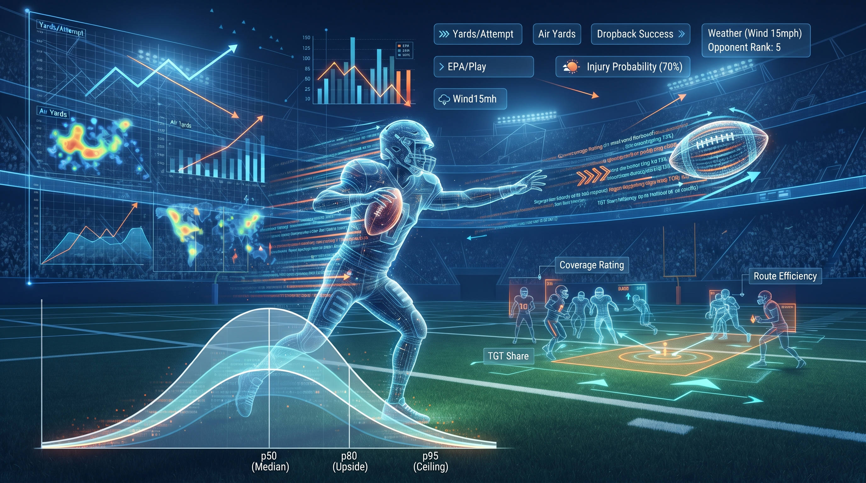
As a pro analyst who builds models for a living, I break down NFL passing yards projections the same way coaches script drives: clear inputs, clean data, and smart adjustments. We are going to translate film notes, pace, weather, and injuries into repeatable numbers, then stress test scenarios so you get realistic medians and upside without guesswork. Building models like this takes a lot of trial and error, but once you find a groove, everything clicks into place. You start seeing why certain numbers move and how small shifts in offensive pacing alter the entire landscape of a game. When scaling these systems into a full-scale sports forecasting platform, organization and automated pipeline management become your best friends.
Building an NFL Passing Yards Projection Model That Bettors Actually Use
When you first sit down to map out an NFL passing model, you realize quickly that raw talent is only half the battle. You have to account for how coaches think, how coordinators adjust at halftime, and how random weather events completely flip a passing script on its head. Most people just look at season long averages and hope for the best, but that is a quick way to lose money. You need a structured approach that weighs every single snap and play call against historical baselines. That is what separates casual fans from people who actually build winning systems using robust predictive sports modeling.
Scope and outcome
What the model covers and what we expect from it
The NFL passing yards projection model is designed to deliver quarterback single-game projections with calibrated uncertainty bands and season-long running totals. The primary outputs are median passing yards per quarterback per game, along with 80th and 95th percentile outcomes for upside tails, plus season-to-date and rest-of-season rolling projections that add up game-level medians and quantify uncertainty. The granularity is team, quarterback, and week, meaning we model the quarterback as the unit linked to his team context and that week's opponent while handling in-season transfers, benchings, and injury substitutions separately to avoid over counting. Use cases include player props for passing yards and completions, daily fantasy sports and fantasy simulations, point spread and totals context since passing implies pace and game script, and internal prioritization at ATSwins for pick confidence and alerts.
Inputs we’ll prioritize
We keep the focus on variables that move pass volume and air yards rather than only focusing on completion percentage. These include team neutral pass rate when win probability is between twenty and eighty percent and the score is within seven points, offensive pace measured by seconds per play and no huddle rate, air yards per attempt and quarterback aDOT, expected points added per dropback and quarterback efficiency indicators, offensive line pass protection signals and pressure rate proxies, receiver route rates, target share, and air yards share, and opponent pass defense splits including allowed aDOT, explosive pass rate allowed, and expected points added per dropback allowed. We also look closely at injury status for quarterbacks, offensive line starters, top receivers, and opposing cornerbacks or safeties, stadium and weather conditions like wind, precipitation, temperature, and domes, late-game trail rate, red-zone pass rate, and pass rate over expected by down and distance.
Keep assumptions transparent
We make sure to model dropbacks rather than just pass attempts because sacks and scrambles are a massive part of the overall play volume story. Neutral pass rate and pace form the true backbone of volume, while quarterback accuracy and connection with receivers translate that volume into actual yards on the field. Injuries and weather are inherently noisy variables, so we inject uncertainty into the model rather than trying to hand wave past them. Opponent adjustments are lagged carefully to prevent overfitting to last week's outlier performance, and small samples are always shrunk using hierarchical or regularized approaches to keep everything stable.
Data and wrangling
Core data stack and what each source provides
Your data stack dictates the ceiling of your entire model. We rely heavily on play-by-play data with expected points added and penalties included, which gives us structured event-level data ideal for tracking pace, neutral pass rate, and drive context. We also lean on reference documentation indexes for reproducibility, game logs and depth charts from public archives for tracking sacks allowed rates, tracking data for route tendencies and separation priors when available, and meteorological APIs for wind and precipitation forecasts aligned directly to stadium locations and kickoff times. Keeping track of stadium types like domes, retractable roofs, and outdoor surfaces is crucial, and you always want to check league schedule feeds to align kick times properly.
ETL pipeline, step by step
The extraction, transformation, and load pipeline starts by ingesting play-by-play files for all completed games through Sunday and Monday nights, pulling team and quarterback level logs, gathering roster status and practice participation reports, and pulling weather forecasts for each specific stadium kickoff window. Step two involves normalizing keys by standardizing player IDs and team abbreviations across different sources and creating a composite team, week, and opponent key. Step three creates weekly aggregates by computing neutral pass rate, pace, early-down pass rate, red-zone pass rate, and pass rate over expected, while aggregating quarterback dropbacks as attempts plus sacks plus scrambles, and summarizing receiver participation through route rates and target shares. Step four handles opponent adjustments by computing allowed metrics over a rolling window with prior-year shrinkage in September to stabilize early numbers. Step five builds injury signals by creating indicators and severity estimates for key offensive and defensive personnel, imputing questionable tags with historical priors. Step six aligns weather snapshots taken within a few hours of kickoff, converting wind speeds into indexes that penalize deeper throw bands. Step seven runs quality checks to validate that active quarterbacks have valid records and confirms that dropback totals balance out. Step eight stores everything in versioned artifact formats like Parquet to maintain complete reproducibility.
Handle bye weeks and opponent adjustments cleanly
Bye weeks require persisting quarterback and team-week rows with clear bye flags, carrying forward rolling features while freezing high-variance metrics like recent target share until the next active game. For opponent adjustments, you must avoid double counting at all costs. When computing team offense metrics conditioned by opponent, always apply out-of-fold logic in backtests so that a team's offensive efficiency isn't artificially boosted by utilizing the exact same game's defensive metrics.
Injury imputation and inactives
Injury status imputation requires converting practice reports like did not participate, limited participation, and full participation alongside game-time decisions into realistic probabilities of playing. If a starting quarterback is listed as doubtful or below a certain threshold to play, you must create a parallel row for the backup quarterback featuring an adjusted neutral pass rate and aDOT based on coordinator history and preseason usage. Within ninety minutes of kickoff, these probabilities must be replaced with definitive in or out statuses, and for receiver injuries, target and air yards shares need to be reallocated to the next men up while capping sudden jumps to historical maximums to prevent unrealistic spikes in the projections.
Weather and kickoff time alignment
Always align your data to local stadium time, especially when dealing with retractable roofs that might change states depending on the weather conditions. Wind speed and gust adjustments must be applied carefully, penalizing deep throw depth profiles much more heavily than short area checkdowns. Precipitation requires a slight downgrade to yards after catch expectations and reduces explosive pass probabilities when heavy rain or snow is actively falling on the field.
Reproducible schema template
Maintaining a clean schema template ensures your features remain organized across weekly runs. Key fields include quarterback identifier, team name, week number, season year, opponent name, home or road indicator, expected dropbacks, expected attempts, expected air yards, neutral pass rate, pace in seconds per play, no huddle rate, quarterback expected points added per dropback, completion percentage over expected, aDOT, receiver route rates, target shares, air share metrics for top pass catchers, offensive line pass block proxies, defense allowed metrics, red-zone pass rate, pass rate over expected across different downs, trail rates, stadium types, weather metrics, injury probabilities, and the target label for training passing yards.
Useful tools
The tooling ecosystem for this kind of modeling is straightforward if you leverage standard data science libraries and storage formats. Data is best handled through specialized sports data packages and weather APIs, while storage relies on partitioned Parquet files for speed and efficiency. Orchestration can be managed with lightweight workflow schedulers running on Sunday nights and pre-kickoff windows, and validation unit tests check row counts and key uniqueness automatically.
Feature engineering
QB efficiency trends
Quarterback efficiency is captured through rolling four-week expected points added per dropback with season-to-date and opponent-adjusted variants, completion percentage over expected to isolate true accuracy from receiver yards after catch, and aDOT to measure throw depth profiles. Interacting quarterback style with receiver separation provides a clear picture of how well a passing game is functioning before the ball is even thrown.
Dropbacks, not just attempts
Predicting expected dropbacks requires combining neutral pass rate, pace, and spread or trail rate proxies. Converting those expected dropbacks into actual pass attempts means subtracting expected sacks and scrambles, where sacks are directly linked to offensive line metrics and opponent pressure generation rates.
Pressure-rate proxies and OL indicators
Offensive line pass blocking is measured through team sack rates allowed on true pass sets alongside quarterback time-to-throw metrics or quick game rates as mitigating factors. Opponent pass rush proxies look at sack rates generated and pressure-related penalties drawn like roughing the passer or holding calls to gauge how much disruption a defensive front can cause on any given snap.
Receiver target and air yards share
Tracking the route rates of top pass catchers reveals how often a player runs a route on team dropbacks. Target share and air yards share rolling averages help identify who the primary reads are, and adding a stacked alpha indicator helps when offenses concentrate a massive chunk of their downfield yardage across just two elite players, which stabilizes overall weekly outcomes.
Situational passing
Red zone pass rate and inside-the-ten pass aggressiveness affect the touchdown versus yardage tradeoff while signaling an overall pass-first mentality. Pass rate over expected by down-distance buckets helps differentiate early-down volume drivers from long third down situations that impact throw depth and sack risks. Late-game trail rate measures the share of snaps a team spends trailing in the second half, because teams that fall behind early almost always throw the ball at a much higher frequency down the stretch.
Environment and schedule
Dome versus outdoor stadium settings and playing surfaces create subtle shifts in performance, with indoor games providing a slight upward lift to throw depth and total yardage. Short-week travel flags from Sunday games to Thursday night matchups tend to lower overall pace and passing aggressiveness for certain coaching staffs, prompting us to apply modest tactical penalties in those spots. Extreme cold and high winds reduce deep throw attempts, while mild rain bumps short passing frequency up a notch.
Opponent coverage tendencies (approximated)
Allowed aDOT serves as a rough signal for defensive shell choices versus press coverage, while explosive pass rates allowed and yards allowed per reception indicate how soft or vulnerable a secondary is in open space. Creating matchup dials for deep-friendly versus deep-suppressing opponents and man-heavy versus zone-lean schemes lets the model understand how a specific defense matches up against a specific passing attack.
Feature checks and practical template
Keeping features honest requires defining strict windows and long-term anchors for every metric in the pipeline. Documenting caps and floors for noisy rates prevents freak data points from breaking the model, and using conservative ramp-up periods for players returning from injury keeps projections grounded in reality rather than wishful thinking.
Modeling choices
Baselines that earn trust
Before throwing heavy machine learning algorithms at the problem, you need to start with transparent baselines that everyone can understand. A rolling mean or median passing yards figure with opponent adjustments provides an immediate sanity check. Expected dropbacks derived from neutral pass rate and pace multiplied by expected yards per attempt give you a baseline that any complex model must comfortably outperform to justify its existence.
Regularized linear models for interpretability
Ridge, Lasso, and Elastic Net regression models are fantastic for passing projections because they let you map attempts drivers, efficiency metrics, environment flags, and injury indicators directly into readable coefficients. The signs and magnitudes make instant sense to analysts and content teams, and built-in shrinkage naturally handles multicollinearity among correlated passing features.
Tree-based ensembles for interactions
Gradient boosted trees like XGBoost and LightGBM excel at capturing complex, non-linear interaction effects such as wind speed multiplying against aDOT, offensive line pressure proxies colliding with elite pass rushes, or receiver route rates interacting with defensive coverage shells. While they offer stellar out-of-sample accuracy, you have to be careful with overfitting and use strict monotonic constraints and early stopping.
Optional Bayesian hierarchical layer
Hierarchical shrinkage across quarterbacks, teams, and coaching strata allows for stable estimates early in the season when sample sizes are inherently sparse. By utilizing quarterback-level intercepts and team-level pass rate priors, the model generates natural posterior distributions that create credible uncertainty intervals to complement traditional quantile regression outputs.
Simulating game scripts with play volume distributions
Simulating individual plays and dropbacks using distributions for pace and pass rate that shift dynamically with point spreads and totals allows you to stress test various outcomes. For each simulation iteration, sampling neutral pass rate, pace, and yards per attempt from bootstrapped distributions lets you record thousands of passing yard totals, generating natural tails for 80th and 95th percentiles that remain robust during blowouts or overtime games.
Uncertainty: quantile regression and calibration
Fitting quantile regression models directly at target percentiles like the 20th, 50th, 80th, and 95th percentages allows the system to learn distributional targets explicitly. Calibrating these predicted quantiles using isotonic regression on validation folds guarantees proper empirical coverage, ensuring your high-end and low-end bands match real-world historical frequencies.
Blending and weekly governance
Per-week blend weights change dynamically depending on the point in the season. Early in the year, you rely more heavily on hierarchical and regularized weights, while midseason shifts toward ensembles and quantile models, and late-season weeks reintroduce heavier shrinkage when injuries pile up across the league. Tracking model versions and feature sets each week maintains complete governance and explainability across the board.
Evaluation and deployment
Backtesting setup
Time-aware backtesting folds are essential to prevent data leakage from creeping into your historical evaluations. Training on the first eight weeks of a season to validate week nine while rolling forward week by week ensures your opponent adjustments only use information that was available prior to kickoff. Holding out entire historical seasons also verifies how well your pipeline generalizes across changing league-wide rules and schedule cycles.
Metrics we report
Model accuracy is tracked through mean absolute error on passing yards, weighted absolute percentage error to scale errors properly across high-volume and low-volume quarterbacks, and calibration scores that measure empirical coverage across the 50th, 80th, and 95th percentiles to ensure your uncertainty bands are statistically sound.
Drift monitoring after injuries or scheme changes
Weekly drift checks compare predicted pass attempts against actual attempts, flagging potential coordinator shifts if the error exceeds two standard deviations two weeks in a row. Tracking per-team residuals on yards per attempt and throw depth catches subtle play-calling pivots before the market fully catches on.
Error dashboards and fast iteration
Error breakdowns categorized by stadium types, weather bins, opponent pass rush tiers, and point spread buckets help identify exactly where the model struggles. Maintaining a known issues log for rapid-fire roster changes, gadget quarterbacks, or garbage-time inflation ensures you can prioritize feature fixes in the next development sprint.
Pregame refresh workflow
The pregame workflow operates on a strict timeline. Three hours before kickoff, injury reports and weather forecasts are refreshed. Ninety minutes prior to game time, active inactives are locked in, roster shares are reallocated, and pass rates are adjusted if a team loses a vital piece. In the final hour, the final weather snapshot is pulled, calibrated quantiles are applied, and clean projections are published to the product.
Documentation, limitations, and transparency
Disclosing model limitations builds long-term trust with users. We openly discuss early-season small-sample volatility, garbage-time inflation on trailing teams, and weather forecast noise that shifts tails more than medians. Documenting data snapshots, maintaining changelogs for feature definitions, and keeping reproducible notebooks guarantees absolute transparency.
Step-by-step: build your first production-ready pipeline
1) Set up data pulls
Schedule automated weekly pulls for play-by-play files, team logs, daily injury practice reports, and weather forecasts leading up to kickoff. Persist all raw data into date-stamped folders to ensure complete auditability if a bug pops up later in the week.
2) Engineer volume drivers
Compute neutral pass rates using strict filters that isolate competitive game scripts where win probability stays between twenty and eighty percent within a touchdown margin. Combine this with pace metrics and second-half trail rates to forecast expected dropbacks accurately.
3) Build efficiency profiles
Calculate rolling four-week and season-to-date expected points added per dropback, completion percentage over expected, air yards per attempt, and receiver route shares to establish a baseline of how efficiently an offense moves the football.
4) Matchup and environment
Incorporate opponent defensive metrics such as allowed aDOT and explosive pass rates, cross-referenced with offensive line pressure rates and stadium environmental factors like wind speeds and dome designations.
5) Injury modeling
Convert practice designations into exact play probabilities, spinning up backup quarterback scenarios if a starter's status is in jeopardy, and reallocating receiver target shares within realistic historical caps when key pass catchers are ruled out.
6) Baseline and ML models
Establish foundational baseline projections, fit regularized linear models for stable medians, train gradient boosted trees for non-linear interactions, and run quantile regression models to capture the full distribution of outcomes.
7) Simulation layer
Sample pace, pass rate, and efficiency metrics across thousands of simulation runs per quarterback-week to extract empirical percentile outcomes and cross-check them against your quantile regression outputs.
8) Backtest and calibrate
Run rolling origin evaluations across historical weeks, report error metrics, and apply isotonic calibration adjustments to ensure predicted probability intervals match actual realized results on the field.
9) Publish and monitor
Publish final median projections and uncertainty bands alongside clear feature attributions highlighting the top drivers for each quarterback, while continuously monitoring residuals across high-wind games and short-week matchups.
Practical tips that save time
Tools and templates
Maintaining structured feature dictionary templates, quick-reference injury status sheets, weather severity classification charts, and model registry logs keeps your workflow organized and prevents chaotic mistakes right before roster locks.
Common pitfalls to avoid
Never use post-game weather observations when training live models, as that introduces severe data leakage. Avoid overweighting a single extreme game script from the previous week, and always account for sacks and scrambles instead of treating pass attempts as the sole indicator of dropback volume.
Quick sanity checks before publishing
Verify that your quarterback median projection sits within fifteen percent of expected attempts multiplied by expected yards per attempt unless a massive weather or matchup flag justifies a major deviation. Ensure upside tails scale appropriately for volatile downfield offenses compared to conservative dink-and-dunk units.
Detailed feature list with why it matters
Volume drivers
Neutral pass rate dictates baseline tendencies, while pace multiplies overall opportunities, and market spreads push game scripts toward higher passing volume when teams fall behind late.
Efficiency drivers
Throw depth profiles and air yards provide the raw material for yardage accumulation, while expected points added and completion percentage capture true quarterback form and scheme fit.
OL and defensive matchup
Pressure rates constrain downfield throwing opportunities, while defensive coverage tendencies define the ceiling of what an opposing secondary allows.
Environment and schedule
Domes provide consistent boosts, high winds suppress deep passing games, and short rest weeks degrade offensive line protection cohesion.
Situational levers
Red-zone pass rates signal overarching philosophies, while pass rates over expected on early downs stabilize overall volume expectations.
How to convert features into projections, end-to-end
Step A: Attempts and dropbacks
Expected dropbacks are calculated using estimated game plays multiplied by neutral pass rate modifiers and script adjustments based on spreads and trail rates. Pass attempts are then derived by subtracting expected sacks and quarterback scrambles based on pressure interactions.
Step B: Yards per attempt
Base yards per attempt figures are pulled from rolling quarterback efficiency profiles and adjusted using matchup multipliers for soft secondaries or heavy pass rushes, alongside weather multipliers that penalize deep throw efficiency in windy conditions.
Step C: Put it together
Median passing yards equal estimated pass attempts multiplied by adjusted yards per attempt. Upside tails are pulled from calibrated quantile models and cross-referenced with game simulations to account for late-breaking weather or injury news.
Step D: Season-long view
Summing game medians across a full schedule while applying a proper variance model preserves uncertainty rather than relying on naive interval additions, giving bettors a realistic look at rest-of-season outcomes.
Examples of usage decisions bettors care about
When looking at player props, if a quarterback's projection sits comfortably above the sportsbook line under calm weather conditions with elite receiver route rates, it presents a very strong over angle. Conversely, if high winds and elite pressure rates depress the 95th percentile outcome, avoiding ladder bets becomes the smart play even if the median projection clears the line. Fade spots against heavily depleted offensive lines on short rest outdoors offer prime opportunities to trim medians and crush high-end tails.
Simple validation playbook you can repeat weekly
Compare your predicted pass attempts against actual box score numbers every Monday morning. If the model misses by more than five attempts without a sudden injury or weather shift, revisit your neutral pass rate and script weights. Track your top deltas against market closing lines to determine whether misses stem from uncaptured injury intelligence, weather changes, or underlying model bias.
Where to find and check inputs quickly
Play-by-play data and expected points added metrics are sourced directly from nflfastR, while documentation indexes are found on nflverse. Game logs, depth charts, and injury reports are available through Pro-Football-Reference, separation metrics come from Next Gen Stats where accessible, and meteorological forecasts are pulled straight from the National Weather Service API.
Bringing it back to ATSwins users
Quantified value is delivered by labeling every quarterback with a median, 80th, and 95th percentile projection alongside the top driving factors behind the numbers. Bettors can easily compare these intervals with sportsbook lines to spot volatile value opportunities. For a complete powerhouse experience, users can seamlessly link their workflow to an advanced sports betting forecasting system available at ATSwins.ai to parse odds and verify value lines instantly.
Conclusion
We centered our entire framework on projecting quarterback passing yards using clean data, pace and pass rate metrics, situational matchups, weather conditions, and game flow simulations. The biggest movers remain expected points added per dropback, pass rate over expected, throw depth, and pressure rates. Building reproducible pipelines, validating against historical data, and keeping uncertainty honest gives you a massive edge. Ready to act? Use ATSwins; ATSwins is an AI-powered sports prediction platform offering data-driven picks, player props, betting splits, and profit tracking across the NFL, NBA, MLB, NHL, and NCAA. Free and paid plans help you make smarter decisions every single day.
Frequently Asked Questions (FAQs) {#faq}
What is an NFL passing yards projection model?
An NFL passing yards projection model is a systematic framework that estimates how many passing yards a quarterback will accumulate in a specific game or across an entire season. It blends offensive pace, pass rate tendencies, quarterback efficiency metrics like expected points added per dropback, throw depth profiles, offensive line pressure rates, opposing defensive coverages, injuries, and weather conditions. The output provides a median expectation alongside percentile ranges that help bettors understand both the most likely outcome and the realistic upside or floor without relying on pure guesswork.
Which inputs matter most for an NFL passing yards projection model?
The most critical inputs driving passing yard projections include expected dropback volume determined by team pace and neutral pass rate, quarterback efficiency metrics like expected points added and completion percentage over expected, receiver route participation and target shares, offensive line pass protection performance against opposing pass rushes, and environmental factors like stadium types and wind speeds. Focusing heavily on volume drivers and efficiency adjustments yields the most reliable projections over the long run.
How do I handle weather and injuries in an NFL passing yards projection model?
Weather conditions should be factored in by checking wind speeds and precipitation forecasts at kickoff, shaving down throw depth and yards per attempt when sustained winds exceed fifteen mph while treating domes as neutral or slightly positive environments. Injuries require reallocating target and air yards shares to backup pass catchers rather than zeroing out production entirely, and adjusting quarterback efficiency downwards when critical pieces along the offensive line or receiving corps are missing from the lineup.
How do I know if my NFL passing yards projection model is any good?
Model performance is best evaluated by tracking mean absolute error and weighted absolute percentage error against closing sportsbook numbers over a large sample of games. Checking whether your predicted percentile bands align with actual realized outcomes ensures your calibration is statistically sound. Reviewing major misses within twenty-four hours to determine whether weather shifts, unexpected injuries, or strange game scripts caused the error helps you patch gaps and continuously improve your pipeline.
How does ATSwins.ai use an NFL passing yards projection model, and what do I get?
At ATSwins.ai, the passing yards projection model feeds directly into a comprehensive sports intelligence platform that tracks pace, pass rate, pressure rates, and matchups to power verified data-driven insights. Members gain access to player props, betting splits, and profit tracking across major North American and collegiate sports leagues through flexible free and paid plans designed to help bettors make smarter, more informed choices.