Championship basketball tightens every single possession, and that is exactly where hard data tells the real story. As a sports analyst who builds predictive software frameworks, I will break down how to quantify matchup edges, calibrate game-by-game odds, and simulate series outcomes. Expect clear steps, transparent assumptions, and practical takeaways you can use before each tip-off and after every major tactical adjustment.
Table Of Contents
- Model Targets and Granularity for NBA Championship Simulations
- Constructing the Predictive Data Pipeline and Contextual Feature Map
- Algorithmic Blending, Optimization, and Historical Backtesting Models
- Monte Carlo Series Simulations and Platform Integration Guide
- Model Transparency, Structural Limitations, and System Reproducibility
- Frequently Asked Questions (FAQs)
Model Targets and Granularity for NBA Championship Simulations
Before writing a single line of code, we lock down our operational scope. The Finals are entirely different from the regular season. The pace drops significantly, benches shrink to core rotations, and coaches lean hard into matchup chess that rarely surfaces during the winter months. Our architecture must reflect these postseason shifts. We define concrete targets and a highly workable predictive granularity, folding in specific basketball constraints from the opening tip.
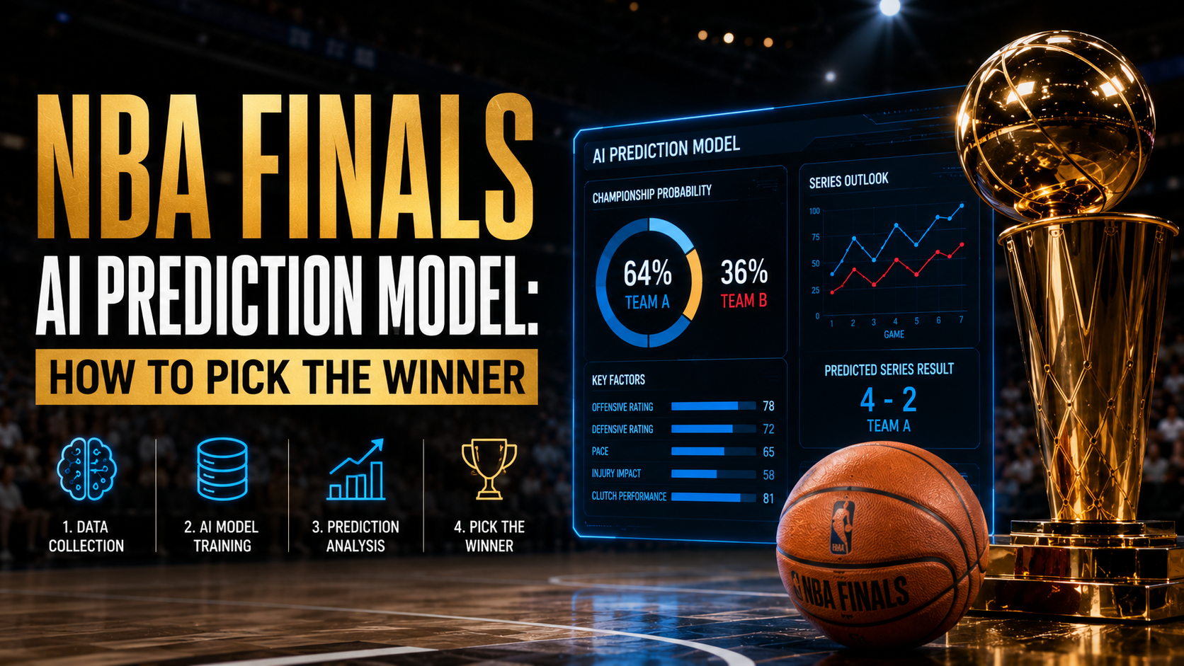
Regarding game-level probability, we compute the absolute win probability for each individual matchup, which translates directly into unvigged moneyline prices. Looking closely at series-level probability, the engine measures the absolute likelihood of a team hoisting the Larry O'Brien trophy, initializing before Game 1 and updating dynamically as fresh data arrives. Finally, the series length distribution layer outputs exact probabilities for the series ending in four, five, six, or seven games, allowing us to find inefficiencies in alternative betting markets.
To maintain computational efficiency while capturing elite tactical adjustments, we split our processing into layers. We ingest micro-data at the possession level, analyzing expected effective field goal percentage based on tracking metrics. However, predicting every individual possession in production introduces immense noise and heavy computation during tight series turnarounds. Instead, we roll these micro-metrics up into stable aggregates normalized per 100 possessions. This powers our primary game-level engine, which pairs pregame team metrics with matchup-specific contextual features like travel miles, rest schedules, and individual defensive assignments.
Standard regular season data fails in June because the style of play undergoes a radical shift. Half-court execution dominates the ledger as transition opportunities dry up. To build a reliable system, our feature weights must heavily favor half-court efficiency over broad transition scoring. Furthermore, rotations compress down to seven or eight players. This makes regularized on-off metrics for top-tier stars far more critical than generic bench production. Whistle sensitivity also alters individual matchups, meaning referee crew tendencies must be tracked alongside free-throw rate sensitivities. Because a seven-game series represents an incredibly small sample size, we partially regularize our championship signals with regular season priors. This prevents our network from overreacting to a single hot shooting night while keeping our predictions firmly grounded in large-sample baseline realities.
Constructing the Predictive Data Pipeline and Contextual Feature Map
An analytical framework is only as good as the underlying data feeds powering its feature store. We aggregate historical data from multiple auditable public platforms to ensure complete consistency.
Our storage layer pulls daily data from reliable athletic endpoints. We ingest play-by-play data, shot locations, and situational tracking logs to build our baseline efficiency metrics. For absolute validation of these core statistics, you can review the official league player database. We also pull multi-year referee logs, game outcomes, and historical lineup information directly from open basketball reference repositories. Comprehensive schedule data provides precise distance measurements for team flights, cross-time-zone travel metrics, and consecutive days of rest. Finally, the ATSwins internal feature store applies custom non-garbage-time filters to remove end-of-quarter noise and clean up rolling performance metrics.
Our model maps specific game properties into distinct feature blocks to separate sustainable execution from pure luck. We contrast expected effective field goal percentage against actual shooting output to capture imminent regression, mapping out spatial shot profiles across various areas of the court. We bin team three-point attempt rates and accuracy trends based on defender contest levels, specifically isolating how defensive schemes alter corner perimeter volume. Our pipeline tracks switch frequencies, pick-and-roll coverage outcomes, and rim deterrence metrics, which reveals how individual rim protectors alter opponent shooting choices near the basket.
We construct rolling identification tags for the top six player combinations, monitoring their shared floor time over trailing spans. The system compiles trailing minute loads and usage spikes to calculate a starter burden index, capturing physical exhaustion during travel turnarounds. We isolate execution data from the final five minutes of close point differentials, adjusting the output based on the strength of the opposing defense. Multi-year referee profiles track free-throw rate variances, technical foul frequencies, and historical home-court whistle bias.
To protect our backtests from selection bias, we implement rolling temporal splits. Every single feature is calculated exclusively using data available prior to that specific game timestamp. Information from Game 4 never leaks into the training matrix for Game 2. When player availability updates surface, we handle the variance through probabilistic scenario trees rather than forcing fixed point estimates. This allows our pipeline to remain perfectly stable across shifting environments.
Algorithmic Blending, Optimization, and Historical Backtesting Models
Our machine learning stack avoids fragile architectures. We utilize a gradient-boosted decision tree framework as our core computational workhorse because of its high predictability and resilience to varying feature scales.
The modeling layer is built on an ensemble framework using tree-based classifiers to capture complex nonlinear interactions across our engineered features, outputting raw, uncalibrated win probabilities. An auxiliary shallow multilayer perceptron neural network with minimal hidden layers processes standardized tracking features, catching deep player interaction variables that decision trees might overlook. Raw model scores often suffer from overconfidence, so we pass our blended outputs through an isotonic regression model to align raw scores with true statistical frequencies.
We use SHAP value analysis to break down exactly why our framework favors a specific side. If a line moves significantly, the system isolates the precise catalyst, whether it is a shifting referee assignment, an altered defensive coverage strategy, or an unpriced rest advantage. This maintains total transparency for every generated prediction.
We validate our predictive models using a strict rolling-origin approach. The framework trains on historical seasons up to a specific year and validates exclusively on the subsequent postseason. We evaluate model performance using Brier scores and log loss metrics to verify absolute probability accuracy rather than simple win-loss records. Furthermore, we test our models against a historical baseline using an unadjusted Elo system to ensure our specialized championship modifiers provide real, measurable analytical value.
Monte Carlo Series Simulations and Platform Integration Guide
Once our game-level probabilities are perfectly calibrated, we feed those metrics into a high-powered simulation engine to project full series outcomes.
Our simulator executes over 50,000 distinct iterations for each championship series. The algorithm takes into account the shifting home-court sequence, potential player suspensions, and physical travel demands. During every individual simulation run, the engine applies random variance draws across our shooting profiles and referee metrics, terminating the loop the exact moment a team secures four victories. This creates a highly accurate series length distribution matrix.
Our simulation platform lets analysts pressure-test specific athletic variables. We simulate lines under the assumption that a crucial rim protector plays limited minutes due to injury management. We restrict opponent three-point percentages to historical floors to observe how a cold shooting stretch impacts series longevity. The engine scales foul frequency variables up or down by a standard deviation to model tight or loose whistle environments.
Every morning of a scheduled game, our pipeline refreshes its feature store by 8:00 AM Eastern time. We ingest updated practice reports, official injury designations, and referee assignments. The system re-calibrates its raw probability metrics, builds our scenario trees, and runs the 50,000 Monte Carlo iterations. The finalized outputs are instantly streamed to the ATSwins.ai interface, providing members with precise edges and recommended bet sizes managed under conservative fractional Kelly Criterion parameters.
Model Transparency, Structural Limitations, and System Reproducibility
Maintaining an analytical edge requires documented tracking, transparent limitations, and a commitment to data integrity. Every feature category is mapped alongside its historical schema snapshots to guarantee total system auditability.
We actively monitor several systemic data traps that can skew automated predictions. Short series often create deceptive statistical noise, so we apply heavy shrinkage modifiers to prevent the model from overvaluing brief hot streaks. The modern explosion of three-point volume can break historical models trained on older eras, meaning we must apply era-aware weights to ensure older physical baselines do not corrupt modern strategic assessments. Late-breaking injury report updates can swing a simulated edge instantly, an issue our pipeline addresses by constantly executing real-time scenario updates up to 60 minutes before tip-off.
Our prediction logs are permanently preserved next to our code repositories, allowing analysts to review historical performance across any past playoff round. To find the true statistical value in these numbers, checking the updated NBA standings helps contextualize regular season data against postseason team drift. We display detailed projection cards, market comparison lines, and dynamic performance splits directly on our main dashboard. Bettors can evaluate these championship edges against historical seasonal baselines, ensuring every betting choice is backed by rigorous, clear statistical modeling.
Frequently Asked Questions (FAQs)
How does the model account for sudden in-series adjustments made by a coach?
The model adapts by treating in-series games as a rolling data pipeline. While it retains large-sample regular season priors to avoid overreaction, it weights recent postseason matchups heavily. If a coach shifts coverage from a traditional drop scheme to a high-frequency switch, the micro-matchup feature layer detects this structural change within a single game. The updated switch frequency numbers are fed directly into the next game's pregame feature array, automatically adjusting the defensive efficiency expectations and moving the baseline line for subsequent games.
Why use a blend of XGBoost and a Neural Network instead of just one advanced model?
We blend these models because they excel at capturing entirely different data patterns. The gradient-boosted tree framework handles structured tabular data exceptionally well, showing high resilience to varying feature scales and protecting the system from overfitting small postseason samples. The shallow multilayer perceptron, meanwhile, is brilliant at discovering hidden high-order interactions between continuous variables, such as the relationship between a team's offensive pace, a starter's trailing usage burden, and a referee crew's average foul call rate. Combining them provides a more robust estimate.
Can this model be used for live, in-game betting as possessions happen?
This specific framework is designed strictly for pregame projections and multi-game series simulations. Live in-game betting requires real-time data ingestion infrastructure capable of processing individual possessions within milliseconds. While our model utilizes possession-level data to build aggregate pregame features, it does not recalculate probabilities live during game action. Trying to force a pregame architecture into a live tracking environment ignores critical micro-variables like active foul trouble, immediate fatigue, and real-time shot heatmaps.
How are player injuries handled if their status is uncertain up until tip-off?
We resolve injury uncertainty by using dynamic, probabilistic scenario trees instead of standard point-blank guesses. If a star player is listed as questionable, our analysts do not guess whether he will play. Instead, we create a multi-branched probability node. One branch simulates the game with the star fully active, a second branch models him playing limited minutes with reduced usage, and a third branch simulates a complete scratch. We assign initial weights to these branches using medical reporting, updating the weights in real-time as official shootaround news breaks.
What is the role of referee analytics in predicting low-sample playoff series?
Officiating tendencies play a massive role in tightening point margins during championship environments. Referee crews possess distinct historical profiles regarding free-throw rates, technical foul frequencies, and home-court whistle variance. Our pipeline tracks these multi-year trends to evaluate how a specific crew interacts with a team's defensive style. If an aggressive, paint-crowding defense is assigned an officiating crew that historically calls a tight whistle, the model increases the projected opponent free-throw rate, directly impacting the game's defensive rating projection.