

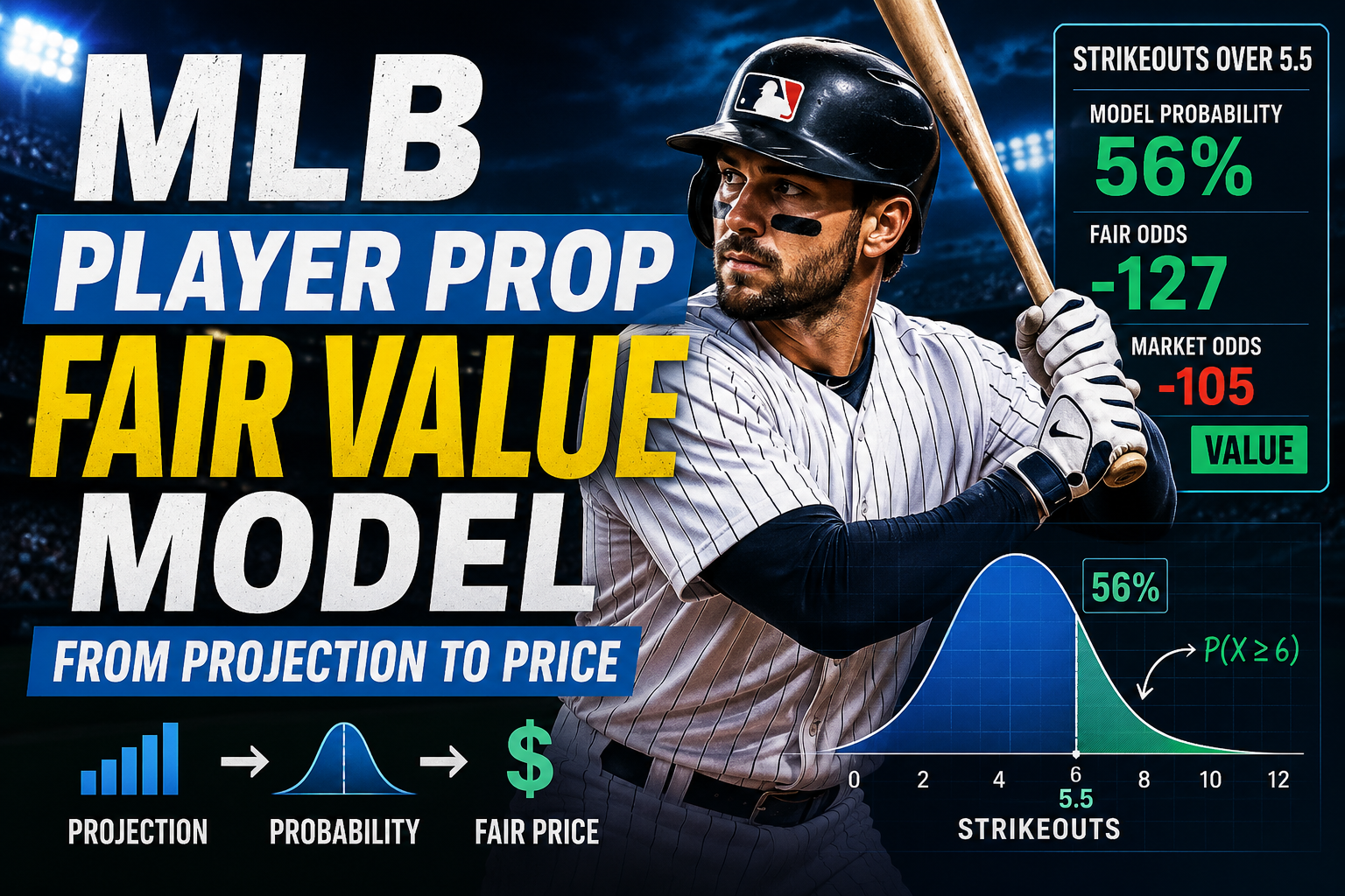
An MLB player prop fair value model estimates what a player prop should be worth based on probability rather than simply following the market price or making a yes-or-no prediction.
That distinction is important. If a model projects a starting pitcher for 6.2 strikeouts, the projection alone does not tell you whether an over 5.5 strikeout prop represents fair value. The more useful question is how often the pitcher is expected to reach six or more strikeouts.
A fair value model attempts to answer that question by combining player performance, matchup conditions, expected playing time, game environment, statistical distributions, and probability calibration. The resulting probability can then be converted into fair odds and compared with the available market price.
This approach applies to many MLB player props, including strikeouts, hits, total bases, walks, home runs, runs, RBIs, and other statistical markets. The goal is not to eliminate uncertainty. It is to measure it more carefully.
Table of Contents
What an MLB Player Prop Fair Value Model Does
The Data Behind an MLB Prop Model
How a Projection Becomes a Probability
How Probability Becomes Fair Odds
Why Model Calibration Matters
Comparing Fair Value With the Market
A Practical MLB Player Prop Example
Where MLB Fair Value Models Can Go Wrong
How ATSwins Fits Into the Modeling Process
Frequently Asked Questions
Conclusion
What an MLB Player Prop Fair Value Model Does
An MLB player prop fair value model is designed to estimate the probability of a particular player prop outcome and determine what price would theoretically correspond to that probability.
That is different from simply predicting a player's expected statistical performance.
Imagine a pitcher is projected to record 6.2 strikeouts. A basic projection system might present 6.2 as its final answer. A more complete fair value model asks what the entire range of possible strikeout outcomes looks like.
The pitcher might have a meaningful chance of recording four strikeouts, another probability of recording five, another probability of recording six, and so forth. The model can use that distribution to determine the probability that the pitcher records at least six strikeouts.
That distinction becomes especially important when the prop line is close to the player's expected performance.
A projection of 6.2 strikeouts does not automatically mean that an over 5.5 strikeout prop has a 62 percent probability of winning. The distribution around the projection matters.
Two pitchers can have the same 6.2 strikeout projection while having very different levels of uncertainty. One may have outcomes concentrated around six or seven strikeouts, while another could have a much wider range.
A useful MLB player prop fair value model therefore focuses on probability distributions rather than relying exclusively on point projections.
The Data Behind an MLB Prop Model
The quality of a fair value model depends heavily on the quality of its inputs.
For pitcher props, a model may consider strikeout rate, opponent strikeout tendencies, pitch mix, velocity, pitch movement, handedness, expected innings, projected pitch count, recent workload, and the quality of opposing hitters.
For hitter props, relevant information can include contact rate, strikeout rate, expected batting average, expected slugging percentage, expected wOBA, quality of contact, launch angle, sprint speed, platoon matchup, batting-order position, and projected plate appearances.
MLB's Statcast system provides detailed information that can be useful for this type of modeling. Statcast tracks measurements such as exit velocity, launch angle, pitch velocity, pitch movement, sprint speed, and other physical characteristics.
Expected statistics are particularly useful because they can provide additional context beyond traditional box-score results. A hitter who has produced poor results despite consistently strong contact may receive a different projection from a model than a player whose recent production has been driven by weaker underlying contact.
Opportunity is another major factor.
A hitter expected to receive five plate appearances has more opportunities to record a hit or total base than the same hitter projected for three plate appearances. Similarly, a starting pitcher projected to face thirty batters has a different strikeout ceiling from one expected to face twenty-four.
This is one reason player prop modeling cannot rely entirely on season averages.
The model needs to understand not only how well the player performs, but also how many opportunities the player is likely to receive.
Game conditions can matter as well. Ballpark characteristics, weather, opponent quality, lineup changes, defensive matchups, bullpen availability, and managerial decisions can all influence the expected distribution of outcomes.
The objective is not to include every possible variable. It is to identify information that meaningfully improves the forecast without making the model excessively sensitive to noise.
How a Projection Becomes a Probability
The most important step in an MLB player prop fair value model is moving from a point projection to an outcome probability.
Consider a hypothetical starting pitcher projected for 6.2 strikeouts.
That projection tells us the model's expected result, but it does not directly answer whether the pitcher is likely to clear a 5.5 strikeout prop.
To answer that question, the model needs an estimated distribution of possible outcomes.
Suppose the model calculates a 56 percent probability that the pitcher records six or more strikeouts.
Now the projection has been converted into a probability that directly relates to the market line.
The model can then determine how often the pitcher is expected to clear the prop under the assumptions being used.
There are different ways to build these distributions.
A statistical model might use a probability distribution appropriate for count data. A machine-learning model might estimate the probability of different outcomes based on historical player and matchup characteristics. A simulation-based model could simulate individual plate appearances and aggregate the results over the expected number of batters faced.
The simulation approach can be particularly useful for MLB because many player props are naturally connected to individual opportunities.
For example, a pitcher strikeout model can estimate the probability of a strikeout against each expected batter and then simulate the expected sequence of plate appearances.
The same concept can be applied to hitters.
Instead of simply saying that a hitter is projected for 1.4 total bases, the model can estimate the probability of zero total bases, one total base, two total bases, three total bases, and four or more total bases.
That creates a much more useful foundation for pricing player props.
How Probability Becomes Fair Odds
Once the model produces a probability, that probability can be converted into a theoretical fair price.
For decimal odds, the basic calculation is:
Fair decimal odds = 1 ÷ probability
If the model estimates a 56 percent probability, the calculation is:
1 ÷ 0.56 = 1.79
The theoretical fair decimal price would therefore be approximately 1.79.
In American odds, a 56 percent probability corresponds to approximately -127.
The purpose of this calculation is not to predict what a sportsbook will offer. It is to determine what the price would look like if the model's probability were treated as the fair probability.
This creates an important distinction between a model's fair price and the market price.
Suppose the model estimates a 56 percent probability for an over 5.5 strikeout prop, while the available market price is -105.
The market price implies a break-even probability of approximately 51.2 percent.
The model therefore estimates a probability roughly 4.8 percentage points higher than the market's implied probability.
That difference may indicate theoretical value according to the model.
It does not mean the outcome is guaranteed.
A player can still finish below the prop line even when the model assigns the over a probability greater than 50 percent. Probability describes likelihood, not certainty.
This is one of the most important concepts in sports analytics.
A fair value model is not designed to tell you what will definitely happen. It is designed to estimate how likely different outcomes are and compare those estimates with available prices.
Why Model Calibration Matters
A model can produce impressive-looking probabilities without actually being well calibrated.
Calibration asks whether predicted probabilities correspond reasonably well with observed outcomes over large samples.
If a model assigns an event a 60 percent probability many times, approximately 60 percent of those events should occur over a sufficiently large and representative sample.
A model that regularly assigns 70 percent probabilities to events that happen only 55 percent of the time has a calibration problem.
This matters because fair odds depend directly on probability.
If the probability is systematically too high, the fair price will also be systematically too aggressive.
That is why evaluating an MLB player prop fair value model requires more than checking how many individual predictions were correct.
Metrics such as Brier score, log loss, calibration curves, and out-of-sample performance can provide a better picture of probability quality.
Historical validation also needs to be designed carefully.
A model predicting an MLB game should only use information that would have been available before that game. Randomly mixing historical games into training and testing datasets can create information leakage and make the model appear more accurate than it actually is.
Walk-forward testing is generally more realistic for sports forecasting because the model is trained on earlier information and then evaluated on subsequent games.
This also makes it possible to monitor model drift.
Baseball changes over time. Pitchers adjust their pitch arsenals. Hitters change swing mechanics. Teams change strategies. League-wide offensive environments shift. Rules and ball characteristics can also affect statistical patterns.
A model that performs well under one set of conditions may require recalibration later.
Comparing Fair Value With the Market
The real analytical value of a fair value model appears when the model's output is compared with an actual market price.
There are three separate concepts to keep in mind.
Model probability represents the model's estimated likelihood of the outcome.
Fair odds represent the theoretical price associated with that probability.
Market odds represent the price currently available.
Keeping these concepts separate prevents a common analytical mistake: assuming that a strong player projection automatically means a strong betting opportunity.
Imagine a hitter has a model probability of 42 percent for recording two or more total bases.
The fair decimal price would be approximately:
1 ÷ 0.42 = 2.38
If the market offers 2.70, the available price is higher than the model's theoretical fair price.
If the market offers 2.10, the available price is lower.
The player's underlying projection has not changed. What changed is the relationship between the model's estimate and the market price.
This is why sports prediction and sports pricing are related but separate disciplines.
A model can correctly identify a player as likely to perform well while still determining that the available price does not offer attractive theoretical value.
Closing-line value can provide another way to evaluate a forecasting process. If model-generated prices consistently compare favorably with the eventual market close, that may provide useful evidence about the quality and timing of the underlying process.
It is still not proof that every individual prediction is correct. Baseball contains substantial short-term variance, and no model can remove that uncertainty.
A Practical MLB Player Prop Example
Consider a hypothetical pitcher facing an opponent with a relatively high strikeout tendency.
The model projects the pitcher for 6.2 strikeouts.
After accounting for the expected workload, opposing hitters, matchup characteristics, and the distribution of possible outcomes, the model estimates a 56 percent probability of recording six or more strikeouts.
The corresponding fair price is approximately -127.
Suppose the market price is -105.
At first glance, the model sees a difference between its estimated fair price and the available market price.
But the analysis should not end there.
The model needs to consider whether the pitcher is expected to maintain a normal workload.
If the pitcher is unexpectedly placed under a pitch-count restriction, the expected number of batters faced could decline.
That would reduce the number of opportunities to generate strikeouts.
The probability distribution could change significantly.
Perhaps the original 56 percent probability falls to 51 percent.
The fair price has now changed.
This demonstrates an important feature of player prop modeling: fair value is conditional on the information available at the time of the forecast.
A model that does not respond appropriately to lineup changes, injuries, workload restrictions, or other relevant information can become outdated quickly.
That is why real-time information and model updating are important components of serious sports forecasting.
Where MLB Fair Value Models Can Go Wrong
Even sophisticated models have limitations.
Data quality is one of the biggest concerns. Incorrect, delayed, or incomplete data can produce an inaccurate projection regardless of how advanced the modeling technique is.
Small samples create another challenge.
A player who has experienced an unusual stretch over a small number of games may not actually have changed as much as the recent statistics suggest. Overreacting to short-term results can cause a model to move too far away from a player's established baseline.
Role uncertainty can also create problems.
A hitter's batting-order position may change. A starting pitcher may have an unexpected workload limitation. A player who normally receives regular playing time may be given a rest day.
These changes can have a meaningful impact on player props.
Model uncertainty is another factor.
Two models can use reasonable assumptions and still produce different probabilities because they weight variables differently or use different approaches to estimating variance.
There is also simple baseball randomness.
A hitter can make excellent contact and record an out. A pitcher can generate weak contact that happens to find a hole. A borderline pitch can become a called strike or a ball depending on the specific circumstances.
One game is not enough to determine whether a probability model is fundamentally correct.
The proper evaluation should happen over larger samples.
That means looking at probability calibration, prediction error, price quality, model stability, and performance across different conditions rather than judging a system by a handful of individual outcomes.
How ATSwins Fits Into the Modeling Process
ATSwins approaches sports forecasting as a probability and modeling problem rather than as a guarantee of specific outcomes.
That philosophy fits naturally with fair value analysis.
The objective is not simply to produce an “over” or “under” recommendation. A more useful process is to estimate player performance, model the distribution of possible outcomes, calculate the probability associated with a particular prop line, convert that probability into a fair price, and then compare it with the market.
ATSwins has published related MLB analysis covering pitcher-versus-hitter matchup modeling, advanced statistics, player props, simulations, and closing-line value.
Those concepts form a connected analytical workflow.
Player data provides the foundation.
Matchup information adjusts the baseline.
Expected opportunity determines how many chances the player is likely to receive.
The outcome distribution estimates the range of possibilities.
Probability calibration tests whether those estimates behave reliably.
Fair pricing converts the probability into a comparable number.
Market comparison shows how the model's estimate differs from the available price.
Ongoing validation determines whether the process continues to perform under changing baseball conditions.
This approach keeps the emphasis on analytical discipline rather than certainty.
For readers using ATSwins for MLB research, fair value modeling provides a useful framework for interpreting player projections and understanding what those projections actually mean.
Conclusion
An MLB player prop fair value model provides a framework for turning player projections into probabilities and probabilities into prices.
The process begins with player performance and expected opportunity. Matchup conditions, Statcast information, lineup context, workload, and other relevant variables can then influence the projection. Instead of stopping at a single projected number, the model estimates a distribution of possible outcomes and determines the probability of clearing a specific prop line.
That probability can be converted into fair odds and compared with the market.
The most important point is that fair value does not mean certainty. A model can estimate a 60 percent probability and still see the outcome fail. What matters is whether the probability is well calibrated and whether the process remains reliable across a meaningful sample.
For MLB analysts, this makes fair value modeling more than a prediction exercise. It becomes a disciplined method for evaluating projections, uncertainty, pricing, and market differences.
ATSwins can be used as part of that broader sports analytics workflow, with the emphasis remaining where it belongs: data, probability, model validation, and informed decision-making.
Frequently Asked Questions
What is an MLB player prop fair value model?
An MLB player prop fair value model estimates the probability of a player reaching a specific statistical outcome and converts that probability into a theoretical fair price. Instead of simply predicting that a player will go over or under a line, the model estimates how frequently the outcome should occur under the available information. This allows analysts to compare a model-generated fair price with a market price.
How is fair value calculated for an MLB player prop?
Fair value starts with an estimated probability. For decimal odds, the basic calculation is one divided by the probability. For example, a 50 percent probability corresponds to fair decimal odds of 2.00. A 56 percent probability corresponds to approximately 1.79 decimal odds or -127 American odds. The calculation provides a theoretical price based on the model's probability rather than the current market.
Is an MLB player projection the same as fair value?
No. A projection and fair value answer different questions. A projection estimates a player's expected statistical performance, such as 6.2 strikeouts. Fair value estimates the probability of reaching a specific prop line and then converts that probability into a price. A strong projection does not automatically mean the market price is favorable because the market may already reflect that expectation.
What data is useful for MLB player prop modeling?
Useful inputs depend on the specific prop. Pitcher strikeout models may use strikeout rate, opponent tendencies, pitch characteristics, projected workload, handedness, and expected batters faced. Hitter models may use contact quality, strikeout rate, expected statistics, platoon matchup, batting-order position, projected plate appearances, ballpark conditions, and other relevant context.
Can an MLB fair value model guarantee profitable results?
No. A fair value model cannot guarantee individual outcomes or consistent profits. Baseball contains substantial random variation, and model probabilities are estimates rather than certainties. A stronger evaluation focuses on calibration, out-of-sample performance, price quality, and results across sufficiently large samples rather than treating individual predictions as guaranteed outcomes.
Why does probability calibration matter for player props?
Calibration matters because fair pricing depends on the accuracy of the probability estimate. If a model consistently assigns probabilities that are too high or too low, its fair prices will also be distorted. A well-calibrated model should have predicted probabilities that broadly correspond with observed frequencies over large, representative samples.