

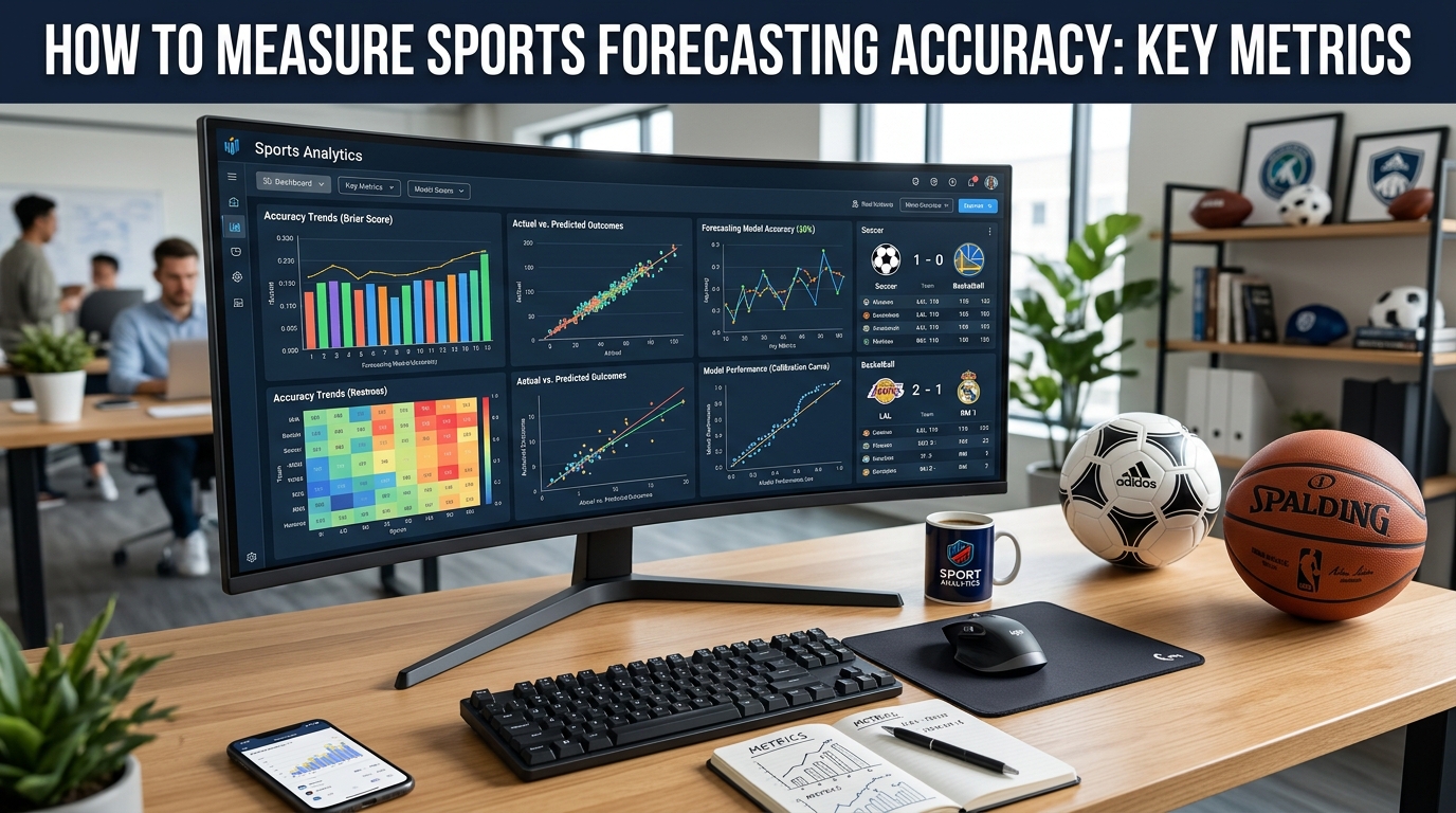
Measuring sports forecasting accuracy requires more than counting how many predictions were correct. A useful evaluation examines whether a model assigns realistic probabilities, how far its projections miss actual results, and whether its performance holds up on games it has never seen before.
The most effective approach combines probability scoring, calibration checks, appropriate error metrics, and comparisons against simple benchmarks. For example, a model that assigns a team a 65% chance of winning should be evaluated across many comparable forecasts, not judged by whether that team wins one particular game. The same principle applies to player projections, point spreads, game totals, and simulated outcomes.
For sports analysts, the goal is to measure forecast quality consistently, identify weaknesses, and distinguish genuine predictive information from ordinary game-to-game variance.
Why Win Percentage Is Not Enough
Win percentage is an intuitive starting point. If a model correctly predicts 58 of 100 game winners, its observed hit rate is 58%. However, this number reveals little about whether the model's underlying probabilities were reliable.
Consider two hypothetical models. The first assigns a favorite a 55% chance of winning and gets the outcome right. The second assigns that same favorite a 95% chance and also gets it right. A simple hit-rate calculation treats both predictions identically, even though the confidence levels are very different.
The distinction becomes clearer when the favorite loses. The first model anticipated a substantial chance of defeat; the second forecast an outcome it considered highly unlikely. An evaluation method that records only wins and losses misses that difference.
Hit rate also depends on the difficulty of the predictions. A model that always favors the strongest teams may accumulate correct picks without identifying which games are unusually competitive or which underdogs have meaningful chances.
Sports forecasting accuracy should therefore be evaluated at several levels. Did the model rank likely winners correctly? Were its probabilities realistic? How close were its numerical projections to the results? Did it outperform reasonable alternatives?
These are separate questions, and no single metric answers all of them.
Brier Score and Log Loss
For forecasts expressed as probabilities, two widely used evaluation metrics are the Brier score and log loss. Both compare predicted probabilities with actual outcomes, but they penalize errors differently.
How the Brier score works
For a binary event, the Brier score is the squared difference between the predicted probability and the observed outcome.
BS = (1/N) × sum of (pᵢ − yᵢ)²
Here, pᵢ is the predicted probability, yᵢ equals 1 if the event occurred and 0 otherwise, and N is the number of forecasts. Lower scores indicate better performance. A perfect binary forecast has a score of zero.
Suppose a model assigns a team a 70% chance of winning. If the team wins, the Brier score for that forecast is (0.70 − 1)² = 0.09. If the team loses, the score is (0.70 − 0)² = 0.49.
The second result receives a larger penalty because the outcome was less consistent with the forecast. However, one loss does not automatically prove the model was poor. A 70% probability still implies that the event will fail to occur about 30% of the time over comparable, well-calibrated forecasts.
For a binary outcome, repeatedly forecasting 50% produces a Brier score of 0.25. That provides a useful reference point, although a more appropriate baseline depends on the sport, event, and prevalence of each outcome.
How log loss works
Log loss evaluates the probability assigned to the outcome that actually occurred. For a binary event:
LL = −(1/N) × sum of [yᵢ ln(pᵢ) + (1 − yᵢ) ln(1 − pᵢ)]
Lower log loss is better. Unlike the Brier score, log loss penalizes extremely confident mistakes particularly heavily.
If a team receives a 90% win probability, a victory contributes approximately 0.105 to log loss. A defeat contributes approximately 2.303. The difference reflects the model's strong claim that defeat was unlikely.
That makes log loss useful when analysts want to discourage exaggerated confidence. It also means that a few highly confident errors can materially affect the average.
The Brier score and log loss complement each other. Neither should be interpreted in isolation, and neither automatically tells an analyst whether a model is profitable or superior to a relevant market benchmark. For further background on sports model evaluation, see this academic review of methodology and evaluation in sports analytics.
Calibration and Reliability
A forecast is calibrated when events assigned a given probability occur at approximately that frequency over a sufficiently large set of comparable predictions.
If a model publishes 500 forecasts at 60%, approximately 300 outcomes would be expected to occur if those forecasts are well calibrated. The realized total will vary, so an exact match is neither necessary nor expected.
Calibration is best examined by grouping forecasts into probability bands. An analyst might compare predictions in the 50–59%, 60–69%, 70–79%, and 80–89% ranges. For each group, calculate the average predicted probability and the observed event frequency.
A reliability diagram plots those values against each other. A well-calibrated model tends to sit near the diagonal, where predicted and observed probabilities match.
| Forecast probability | Observed frequency | Interpretation |
|---|---|---|
| 50–59% | 55% | Reasonably aligned |
| 60–69% | 58% | Possible overconfidence |
| 70–79% | 71% | Reasonably aligned |
| 80–89% | 73% | Potential overconfidence |
The final group deserves attention: outcomes occur less frequently than the forecasts suggest. Yet analysts should check how many predictions fall into that band before drawing conclusions. A group containing 15 forecasts is less informative than one containing several hundred.
Expected calibration error (ECE) summarizes differences between predicted probabilities and observed frequencies across groups. It can be useful for monitoring, but its value depends on how the groups are constructed. Different bin widths can produce different results, and a single summary may hide problems in particular probability ranges.
Calibration also does not measure everything. A model that predicts 50% for every game could be calibrated overall but offer little ability to distinguish likely winners from underdogs. Strong forecasting requires realistic probabilities and useful separation between events with different chances.
Choosing the Right Error Metric
The correct metric depends on what the model predicts. A game winner, a point margin, and a player's rushing yards are different statistical targets. Evaluating all three with the same score would obscure important differences.
| Forecast target | Useful metrics | What they measure |
|---|---|---|
| Win, loss, or over/under | Brier score, log loss | Quality of assigned probabilities |
| Game margin or total | MAE, RMSE | Size of numerical errors |
| Player statistics | MAE, RMSE, distributional scores | Projection accuracy and uncertainty |
| Full outcome distribution | CRPS or suitable distributional scores | Quality of the predicted distribution |
| Ranking teams or outcomes | AUC or ranking metrics | Ability to order outcomes by risk or likelihood |
Mean absolute error (MAE) is the average absolute difference between a projection and the result. If a model forecasts a 24-point team score and the team scores 27, the absolute error is three points.
Root mean squared error (RMSE) squares each error before averaging and then takes the square root. Because larger errors receive greater weight, RMSE is especially useful when major misses matter more than several small ones.
For a player projected to record 72 rushing yards, an actual total of 60 creates an absolute error of 12 yards. Across a large sample, MAE indicates the typical size of projection errors. RMSE highlights whether the model also produces occasional large misses.
When a model predicts a complete probability distribution rather than a single number, distributional scoring rules such as the continuous ranked probability score (CRPS) may be more informative. They assess the forecast distribution against the observed outcome.
AUC, meanwhile, measures ranking discrimination rather than probability calibration. A high AUC does not guarantee that a model's stated 70% probabilities occur 70% of the time.
The practical rule is straightforward: choose metrics that match the forecast's intended use, and report complementary measures when one score leaves important questions unanswered.
Test Models Out of Sample
A model can look excellent on historical data and still perform poorly on future games. This often happens when it learns patterns specific to the sample used to develop it rather than relationships that generalize.
Out-of-sample testing measures performance on observations that were not used to fit the model. In sports, a time-aware test is usually more realistic than randomly splitting games across the full season.
For example, a model could be trained on games from earlier seasons, validated on a later period, and tested on an even more recent period. The test set should remain separate until model choices are finalized.
Rolling-origin evaluation provides another useful approach. Train the model using data available up to a particular date, forecast the next set of games, record the results, and advance the cutoff. Repeating this process simulates how the model would operate in practice.
This method helps prevent data leakage: the accidental use of information that would not have been available when a forecast was issued. Examples include using final injury reports in a sports prediction supposedly made before those reports were released, or incorporating closing odds into a forecast timestamped earlier in the day.
A reliable evaluation should preserve the original prediction, publication timestamp, model version, relevant market line, and eventual outcome. Forecasts should not be silently replaced after the result becomes known.
This matters because model performance can change as teams, player roles, coaching strategies, and league conditions change. A strong historical score is evidence, not a guarantee of future performance.
Compare Forecasts With Benchmarks
A metric is easier to interpret when it has a fair comparison point. A Brier score of 0.22, for instance, does not establish that a model is useful without context.
Start with a simple baseline. Depending on the sport and target, that might be a constant probability, a historical league average, a basic rating system, or a model that uses only home advantage and team strength.
For market-related forecasts, compare against market-implied probabilities for the same events and at a clearly defined time. When using bookmaker odds, account for the margin, or vig, before interpreting prices as probabilities. Raw implied probabilities from both sides of a market generally sum to more than 100%.
Use the same event set, settlement rules, and forecast cutoff for each method. If one model is evaluated on all games but the baseline excludes difficult matchups, the comparison is not meaningful.
Analysts should also separate predictive accuracy from financial performance. A model may achieve a good Brier score without generating positive returns after prices, fees, and execution constraints. Conversely, a profitable short run may be driven by variance rather than lasting predictive skill.
Closing-line value (CLV) provides another diagnostic in betting-related analysis. It examines whether a selected price compares favorably with the closing market price, using a consistent definition of the market and its margin. It is not a substitute for probability scoring or realized returns, but it can add context about price evaluation.
Build a Repeatable Evaluation Process
A useful forecasting report should make it possible to understand what was predicted, how it was graded, and where performance is strongest or weakest.
Begin by defining the target. Specify whether a prediction concerns the outright winner, a spread, a total, or a player statistic. Record the probability or projection before the event and document the information available at that time.
Next, select a primary score and a complementary diagnostic. For binary probabilities, Brier score or log loss can serve as the main metric, with calibration plots explaining the pattern of errors. For numerical projections, report MAE or RMSE. If uncertainty ranges are issued, measure interval coverage as well: an 80% prediction interval should contain roughly 80% of outcomes over a sufficiently large and relevant sample if it is well calibrated.
Then segment the results. Compare performance by sport, market type, probability band, and forecast timing. A model might perform well on game winners but struggle with player props, or remain reliable before lineup announcements but deteriorate when late news arrives.
The same approach applies to simulations. If a model simulates a game thousands of times and estimates a team has a 62% chance of winning, the simulation count alone does not establish forecast quality. The estimate must still be tested against real outcomes and compared with appropriate baselines. More simulations reduce Monte Carlo sampling noise, but they do not automatically correct faulty assumptions or poor input data.
Finally, track uncertainty around the evaluation itself. Small samples produce noisy estimates, particularly for high-confidence forecasts and less common events. Confidence intervals, repeated time-based tests, and consistent reporting make it harder to mistake random fluctuations for meaningful improvement.
For a broader view of the modeling process, ATSwins.ai readers can also consult its related coverage of sports prediction variance, machine learning sports predictions, and AI sports insights.
What Accurate Forecasting Really Means
The best sports forecasting model is not necessarily the one with the highest headline hit rate. It is the one whose outputs stand up to appropriate testing, whose probabilities are reasonably calibrated, and whose performance compares favorably with relevant alternatives.
That requires more than collecting final scores. Analysts need timestamped forecasts, suitable metrics, honest baselines, and enough observations to distinguish persistent patterns from ordinary variance. They must also recognize that model quality can differ between sports, markets, and prediction horizons.
For teams evaluating analytical systems, a repeatable measurement process makes weaknesses visible before unsupported claims become conclusions. It also provides a sounder basis for improving inputs, recalibrating probabilities, and deciding which model outputs deserve further investigation.
ATSwins.ai focuses on data-driven sports forecasting and statistical analysis. Use the same disciplined approach when assessing any forecast: examine the probability, test the record, compare it fairly, and treat uncertainty as part of the result.
Frequently Asked Questions
What is the best metric for sports forecasting accuracy?
There is no single best metric for every forecast. Brier score and log loss are useful for binary probabilities, while MAE and RMSE measure errors in numerical projections. Calibration checks whether predicted probabilities align with observed frequencies. A strong evaluation usually combines a primary score with complementary diagnostics and an appropriate baseline.
Is win percentage enough to evaluate a sports prediction model?
No. Win percentage records whether predictions were correct but ignores the confidence attached to them. A model that assigns a 90% chance to an outcome should be evaluated differently from one assigning 52%. Probability scoring and calibration reveal whether confidence levels are realistic, while out-of-sample tests establish whether the results generalize.
How many predictions are needed to measure accuracy reliably?
The answer depends on the outcome frequency, probability range, and level of precision required. A few dozen games may reveal obvious data problems but rarely establish stable performance across multiple categories. Hundreds or thousands of observations can provide stronger evidence, although rare events and high-confidence predictions may still have substantial uncertainty. Report sample sizes alongside metrics.
What is the difference between accuracy and calibration?
Accuracy often refers to the proportion of categorical predictions that are correct. Calibration describes whether events forecast at a given probability occur at approximately that rate. A model can select many winners but be overconfident, or have reasonable calibration while doing little to distinguish strong favorites from close contests. Both properties matter, but they measure different things.
Does a better forecasting score mean a model will be profitable?
Not necessarily. Predictive scores assess forecasts against outcomes, whereas profitability depends on the prices available, transaction costs, market efficiency, and the decisions made using those forecasts. A model must be evaluated against relevant market probabilities and realistic execution assumptions before financial conclusions can be justified.