Implied probability is the secret sauce that turns standard sportsbook odds into clean, usable percentages that you can actually test, calibrate, and bet on. If you have ever wondered how to convert betting odds to percentages, it is essentially the process of turning a price into a raw chance. As someone who works as a pro sports analyst utilizing AI models, I rely on this process daily to strip away the noise and find true value. It is all about removing that annoying vigorish, comparing my model’s calculated edge to the market, and sizing my bets with actual intelligence rather than just guessing. If you can learn to read and master implied probability, you are going to find much steadier returns and, more importantly, a lot fewer nasty surprises when your bets go sideways. It is a fundamental skill that separates the people who treat betting like a hobby from those who are trying to treat it like a serious investment.
Implied probability basics
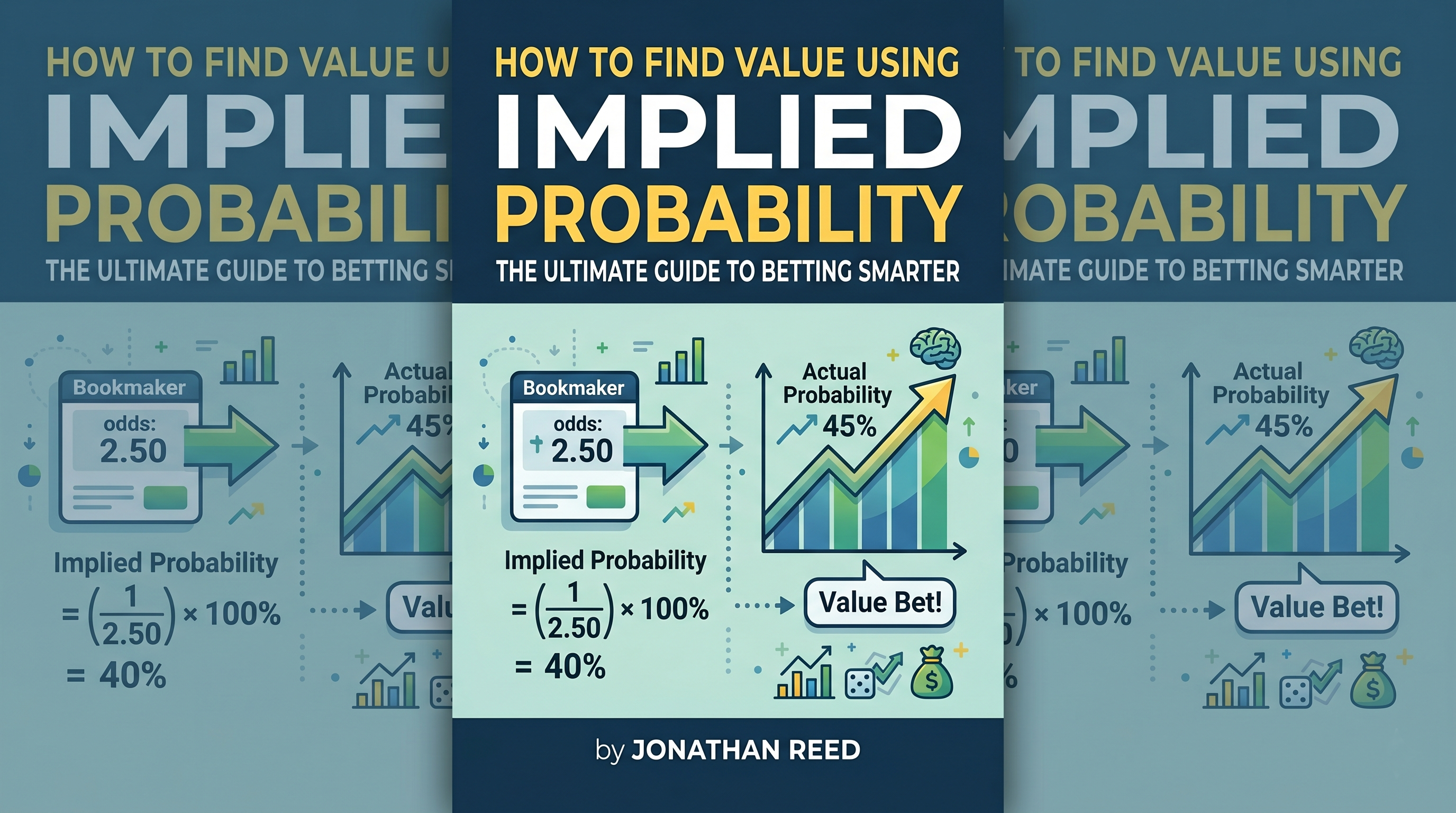
When you look at a sportsbook, every single line you see is effectively a statement of a percentage chance. Implied probability is just that percentage expressed directly from the odds. If you see a moneyline listed at -120, the book is essentially telling you that this specific outcome happens about 54.55 percent of the time before they add their cut. Once you get comfortable translating any price—whether it is a moneyline, a spread, or a total—into a percentage, you are suddenly able to compare it directly to your own model’s percentage. That is the whole game. You convert the price first, then you compare it to your number. Do not skip the math, because the math is the only thing keeping you from making emotional mistakes.
You will need to memorize a few quick conversions that you will use every single day. If you are working with decimal odds, the implied probability is simply one divided by the decimal. For American odds, if the number is positive, the formula is one hundred divided by the odds plus one hundred. If the number is negative, the formula is the absolute value of the odds divided by the odds plus one hundred. For fractional odds, you take the denominator and divide it by the sum of the numerator and the denominator. A few fast examples make this easier to picture. A decimal of 2.40 is one divided by 2.40, which equals 41.67 percent. American -120 is 120 divided by 220, which gives you 54.55 percent. American +150 is 100 divided by 250, resulting in 40.00 percent. Finally, fractional odds of 5/2 are 2 divided by 7, which is 28.57 percent.
The break-even rate is effectively the implied probability. If your model’s win probability is higher than that break-even number, and the math holds up after you remove the juice, you have found a real value edge. A very tight way to remember this for your daily workflow is simple. If your model probability is greater than the market implied probability without the vig, value exists. If your model probability is less than that market number, it is a negative expectation in the long term, and you should walk away.
Remove the vig to see true prices
Sportsbooks always add a margin, which we call the vig or the overround, so the sum of implied probabilities across all outcomes is always going to be greater than 100 percent. That excess is where the book makes its money. If you do not strip that vig out, you are going to confuse fake value, which is just margin distribution, with real value, which is a genuine mispricing relative to the true market.
For two-way markets like spreads and totals, this is pretty easy to handle. Suppose both sides of a game are listed at -110. Each side’s implied probability is 110 divided by 210, which is 52.38 percent. The sum of those two sides is 104.76 percent. That extra 4.76 percent is the book’s margin. You find the no-vig probability by normalizing each side, which means taking the individual implied percentage and dividing it by the total sum of all percentages. So, 52.38 percent divided by 104.76 percent leaves you with 50 percent on each side.
Multi-way markets like soccer games, where there is a draw, or group winner futures, require the exact same normalization approach. If you have decimal prices like home at 2.50, draw at 3.10, and away at 3.00, those represent 40 percent, 32.26 percent, and 33.33 percent, respectively. The sum is 105.59 percent, meaning the overround is 5.59 percent. To get your no-vig probabilities, you take each of those values and divide them by 105.59 percent. The home side becomes 37.89 percent, the draw is 30.55 percent, and the away side is 31.57 percent. If you compare your model to the raw numbers, you will overstate your edge significantly. Always normalize first.
There are a few extra nuances here that most people miss. While two-way markets are straightforward, the margin per leg often differs in multi-way boards. You should always de-vig leg by leg from the total implied sum. Also, be aware that in player props and niche markets, the book can load more margin onto one side specifically. Removing the vig by total-sum normalization is the simplest fix, but you have to be aware that some props have asymmetric exposure and limits that influence that margin. If both sides of a two-way prop are -115 and -105, the juice is not split equally. Always compute the leg-specific implied percentage and then normalize. Lastly, consider your timing. If you are doing this live or midweek, remember that the overround can shift as limits rise. For a fair comparison to your model’s historical performance, you need to use consistent timing, whether that is the open, the mid-point, or the close, and you have to stick with it.
Turn probabilities into value
Once you have your model probability and the market’s no-vig probability, you can finally size up the opportunity using expected value. Learning expected value betting for beginners is about realizing that math does not care about your gut feelings; it only cares about the long-run average. In decimal odds, the standard expected value per one dollar stake is the model probability multiplied by the decimal odds, minus the quantity of one minus the model probability. This formula is vital. If the result is greater than zero, the bet makes money in expectation across many repeats. If it is less than or equal to zero, you should pass. Even if it wins today, the math is against you long-term.
You can also cross-check this with the break-even threshold, which is simply one divided by the decimal odds. If your model probability is higher than one divided by the odds, the bet has positive expected value. Both tests tell you the same thing, but the expected value formula gives you a better sense of the magnitude of your edge. I personally prefer to use the net version of the formula, which allows you to understand exactly how to calculate expected value in sports betting by taking the model probability multiplied by the decimal odds minus one, then minus the quantity of one minus the model probability. This shows you the net profit expectation per dollar staked.
Only flag positive expected value bets for consideration. I recommend adding a margin-of-safety rule, where if your net expected value is less than two percent, or your model’s advantage is less than 1.5 to 2 percentage points over the no-vig price, you should pass. Tiny theoretical edges can easily be eaten by bad execution, slower lines, or data errors. You want to look for stable signals and objective checks. Closing line movement is the gold standard here. If you consistently beat the closing number, your process is generally sound. Record the open versus the close on every single wager. A simple closing line value metric is the difference between your price and the closing price in cents for American odds, or in implied percentage points after you de-vig.
For any bet, you should ask yourself if your calibrated model probability is clearly above the break-even rate. If the answer is barely clearing it, you should size smaller or just don’t bet at all. Value is extremely price-sensitive. For the same opinion, +120 at one book is valuable, but +110 is not. You have to shop for the best line every single time. Track your performance the right way by logging every bet with the model probability, the market no-vig probability, the stake, the expected value, and the book price at the time of the bet. Your goal is not to win every bet, as short-term wins or losses are noisy. Your goal is to see if your edges translate to beating the market over thousands of bets.
Build and calibrate your %
Your edge comes from a probability estimate that is better than the market’s no-vig price. That requires a model that is well-calibrated and robust. Whether you are working on NFL, NBA, MLB, NHL, or NCAA markets, the path is roughly the same. You need to consider team performance and pace, which means looking at things like possessions, plays per game, and overall tempo. You need efficiency metrics like EPA per play, offensive and defensive ratings, and expected goals. You have to account for player availability, including injuries, minutes, snaps, and pitcher or goalie impact. Matchups are critical, such as scheme versus scheme, handedness splits, and coverage tendencies. Finally, don’t ignore the external factors like rest, travel, and market signals like opener versus current prices.
A baseline workflow starts with defining your target and the time slice you are looking at. Are you looking at moneyline win probability, spread cover probability, or prop over probability? You must fix a time-of-day snapshot for your features and labels to keep your data clean. You have to prepare your training data honestly. Train on historical games with features that were available at the same time you would have actually placed the bet. Avoid data leakage, meaning no post-game stats and no closing lines if you are predicting at the open.
Start with a simple model. Logistic regression, gradient boosted trees, or a well-tuned random forest are great starting points. Keep your feature count manageable, because more features are not always better. Evaluate using proper scoring rules like the Brier score, which is the mean squared error of probabilities, or log loss, which penalizes overconfident wrong picks. These are great for calibration. Create reliability plots where you group your predictions into bins and plot predicted versus observed frequencies.
Calibrate your probabilities using isotonic regression or Platt scaling to align your outputs with reality so that 60 percent actually means 60 percent in the long run. Refit your calibration on an out-of-sample validation set to avoid bias. When you backtest, make sure you are testing the decision rule, not just the model. Use walk-forward testing, where you roll through seasons chronologically. Only simulate betting when your edge is above your threshold, such as 1.5 to 2.5 percentage points. Record your simulated return on investment, your drawdowns, and your closing line value. Finally, track your error by market type and timeframe. You might be strong on sides but weak on totals, or vice versa.
ATSwins is designed to help with this heavy lifting. The platform’s AI-driven probabilities and projections give you a solid starting point that you can validate against the market. If you are using your own model, you can still lean on ATSwins for fast context like injury updates, betting splits, and player prop baselines. It speeds up the conversion and comparison cycle without losing your personal rigor. Explore the projections and splits on the ATSwins sports intelligence tool to get an edge on the daily slate.
Bankroll and execution
Edges are incredibly fragile if you bet too big or too randomly. You need a consistent bankroll plan and a repeatable routine to keep you in the game through the inevitable swings of variance. The Kelly criterion is the go-to method for maximizing long-run growth for a known edge. The standard formula for decimal odds involves taking your net odds and your model probability to find the optimal fraction of your bankroll to wager. If your calculated fraction is less than or equal to zero, you skip the bet. If it is greater than zero, you stake that fraction of your bankroll. For practical use, most people take a fraction of Kelly, like 25 to 50 percent, to reduce volatility. Full Kelly is almost always too aggressive for the average bettor.
You should cap your stake volatility. Set a hard maximum stake per bet, for example, one to two percent of your bankroll, and a daily cap. Even with a consistent edge, losing streaks happen. Do not try to use Martingale strategies or start chasing losses because you are tilted. Your edge is statistical, not guaranteed.
Log your closing line value and your outcomes religiously. For each bet, record your price, the closing price, and convert both into no-vig implied probabilities. Over time, a positive average closing line value is the best indicator that you are finding real value in the market. Automate your conversions and alerts as much as you can. Use a spreadsheet or a simple script to handle the odds-to-implied-probability-to-no-vig-to-expected-value pipeline. This lets you apply your staking rule immediately and flag plays that meet your thresholds.
Accept that variance is a part of the deal and stick to your process. Short-term swings are completely normal. Your job is to put repeatable positive expected value tickets into the market. Scale your bankroll as your confidence and your bankroll grow, but do not scale simply because you had one hot week. Respect book limits and local laws. Do not attempt to use gray tactics, because books will eventually limit or close your account. You can still win with small limits by focusing on consistency, line shopping, and niche markets where your model is strongest. Hold accounts at multiple shops so you can shop for lines, as reduced juice at -105 can turn a marginal pass into a strong positive expected value bet.
ATSwins can help you with this tracking. The platform’s picks and player props come with probabilities and historical performance so you can compare your model’s view against a data-driven baseline, then log your bets and evaluate your return on investment over time. If you are building your own workflow, it is still very useful to have a second, neutral set of numbers nearby. See the projections and profit tools on the ATSwins AI-powered projections page. For ongoing education and updates, check the latest pieces in the ATSwins news archive to stay ahead of the curve.
Handy resources
When you need formulas, examples, or a deeper background on these concepts, certain resources are invaluable. For implied probability basics and formulas, Investopedia’s overview is clean and practical. You can also look at Wikipedia for broader context and notation regarding implied probability. For understanding overround and removing the vig, Wikipedia’s entry on overround explains the margin math in multi-way markets quite well. Investopedia also has a very straightforward page on vigorish and how books build their margin.
For bankroll management, Investopedia covers the Kelly criterion with clear examples. Wikipedia’s entry on the Kelly criterion provides the math and the trade-offs, which is useful if you want to understand why using fractional Kelly is so common. If you are interested in probability calibration and evaluation, the scikit-learn documentation is excellent. Their page on probability calibration includes information on isotonic and Platt scaling with helpful usage notes. For scoring rules, look up Brier score and log loss on Wikipedia or the scikit-learn metrics module.
If you are building your own personal toolkit, I have a few tips. Keep a lightweight odds-conversion sheet where you can paste prices in quickly. Make sure to add a market group field so the total implied probability sums correctly for both two-way and multi-way markets. Create a small expected value calculator tab with the columns mentioned earlier. Add your Kelly fraction and maximum stake rules as cells that you can tweak. Archive every single day’s bets and model outputs. You want the ability to run back-tests on your own decisions later because your future self will thank you.
Implied probability: step-by-step workflow checklist
Use this daily routine to find real value and avoid amateur mistakes. First, gather your lines. Pull current prices for your target markets, including moneylines, spreads, totals, and props. For each market, list every outcome and its corresponding odds. Second, convert those odds to implied probabilities based on their format. Third, remove the vig by summing those percentages and dividing each leg’s individual probability by that total sum to get your no-vig probabilities. You can optionally convert those no-vig probabilities back to fair decimal odds for a better intuitive sense of the price. Fourth, overlay your model by generating your own win probability for each outcome using your latest model snapshot. Make sure you confirm that your model is actually calibrated. Fifth, compare and compute your expected value. Calculate your net expected value using the formula provided earlier and cross-check it with the break-even one divided by the decimal odds and your margin-of-safety threshold. Sixth, decide and size your bets. Only consider bets with positive expected value and a sufficient edge over the no-vig probability. Apply fractional Kelly with hard caps like a maximum of one to two percent of your bankroll per play. Seventh, execute your bet by shopping the lines to place it at the absolute best price available. Note the book, the timestamp, and the price. Eighth, track and learn. Log your result, the closing price, your closing line value, and the expected value. Update your bankroll accordingly. Review your performance weekly to see where your edges are concentrated and whether you are consistently beating the close. Adjust your thresholds if your realized return on investment diverges from your expected values.
Common pitfalls to avoid
These are the mistakes I see most often when onboarding new bettors to implied probability workflows. The most common error is comparing model probabilities directly to with-vig prices. You must normalize first, or you will think you have significantly more edge than you actually do. Another issue is using uncalibrated model outputs. A classifier’s raw score is not a probability unless it is calibrated. Sixty percent must mean about sixty percent in the real world, or your math will be off.
Chasing noise is another trap. Props and micro-markets can have asymmetric margins and thin liquidity. Do the math, but be realistic about the fill and the limits. Do not oversize on small edges. The Kelly criterion assumes perfect probabilities and infinite repetitions, but real life has model error and changing markets, so you should always use fractional Kelly or fixed stakes to be safe. Ignoring the closing line value is a major warning sign. If you rarely beat the market by the close, your edge likely isn’t real, or your timing is off. Finally, avoid survivorship bias in your backtests. Do not build features from end-of-day data if you are betting in the morning. If you used closing lines to pick games in your backtests, that is a classic case of data leakage.
Applying the process across leagues
A bit of practical nuance is required for every sport. In the NFL, markets are generally efficient late in the week. Edges often come from injury and role clarity, whether earlier in the week, or from alternate lines where books tend to overprice certainty. Model variables for football should include EPA per play, success rates, pressure rates, receiver and corner matchups, and travel context. In the NBA, player availability drives nearly all of the variance. You must keep a live injury model and adjust for minutes projections and pace changes. Totals can move a lot, so you have to be fast when news drops. Calibration is crucial here because of late scratches.
For MLB, pitcher models are king. Use pitch-level metrics like called strike and whiff rate, expected weighted on-base average, bullpen fatigue, park factors, and weather. First-five-inning markets often have much cleaner edges than full-game lines. In the NHL, goalie confirmation matters immensely. Incorporate team expected goals rates, pace, and special teams statistics. Always watch for travel clusters. For NCAA football and basketball, data quality varies, so priors like power ratings play a much larger role. Calibrate by conference and always adjust for garbage-time effects. Across all of these, the common thread is doing the conversions, removing the vig, and comparing to a calibrated model probability. If you are using ATSwins, you can quickly check our projections and betting splits as a context layer, then apply your own thresholds. When you want to see how others are approaching a slate or want a second opinion, browse the recent posts in the ATSwins archive.
Quick reference formulas
Keep these handy in your worksheet: For implied probability, if you have decimal odds, the probability is one divided by the decimal. For American plus odds, it is one hundred divided by the odds plus one hundred. For American minus odds, it is the odds divided by the odds plus one hundred. For fractional odds, it is the second number divided by the sum of both numbers. To remove the vig, sum all implied probabilities to get S, then divide each individual probability by S to get the no-vig probability. Your break-even rate is simply one divided by the decimal odds. Your net expected value per dollar staked is your model probability multiplied by the decimal odds minus one, then minus the quantity of one minus your model probability. The fractional Kelly formula uses net odds b equal to decimal odds minus one, with the fraction being b times your model probability minus the quantity of one minus your model probability, all divided by b. Small, repeatable edges add up when the math is honest and your probability is well-calibrated. The math is not flashy, but it is exactly what separates real value from a simple gut feel.
Conclusion
We turned odds into implied probabilities, removed the vig, and hunted only for positive expected value edges. The key takeaways are to convert your odds fast, normalize your markets, always check your break-even rates, manage your bankroll with fractional Kelly, start small, log your results, and track your return on investment and closing line value. Use ATSwins, an AI-powered sports prediction platform offering data-driven picks, player props, betting splits, and profit tracking across the NFL, NBA, MLB, NHL, and NCAA. Their free and paid plans give bettors the insights and guides they need to make smarter and more informed decisions. By following this disciplined process, you turn sports betting from a random gamble into a regular exercise in probability and value recognition.
Frequently Asked Questions (FAQs)
What does how to find value using implied probability - bet smarter actually mean?
It means turning betting odds into clear percentages, then comparing those numbers to your own expectation so you only stake when the edge is real. In practice, this is a cycle of converting odds to implied probability, removing the vig, comparing your model’s probability to the no-vig market, and betting only when your edge is positive. Odds are just prices, and implied probability turns them into simple chances you can test. If you are new, it is totally okay to start small and build from there.
How do I convert odds to implied probability so I can how to find value using implied probability - bet smarter?
Quick conversions you will use daily include decimal odds like 1.80, which is one divided by 1.80, giving you 55.56 percent. For American odds like +150, you do 100 divided by 250 for 40 percent. For -150, you do 150 divided by 250 for 60 percent. For fractional odds like 5/2, you do two divided by seven for 28.57 percent. The break-even probability is always one divided by the decimal odds. If your model says the real chance is higher than the break-even, you have potential value.
How do I remove the vig to really learn how to find value using implied probability - bet smarter?
Sportsbooks build in a margin, so raw implied probabilities usually sum to more than 100 percent. To normalize them, convert each price to an implied probability, add them up, and then divide each individual side by that total sum. This gives you the no-vig probability for each side. You then compare your model’s percentage to these no-vig numbers, not the juiced ones. Then, you estimate the expected value by multiplying your model probability by the decimal odds and subtracting the probability of losing. Only fire when the expected value is positive.
What simple tools help with how to find value using implied probability - bet smarter day to day?
You do not need fancy stuff to start. Use spreadsheets to build converters, no-vig calculators, and expected value tools in Google Sheets or Excel. Use a calculator to check your math. Pull data context from reputable sports reference sites for pace, injuries, and matchups. If you estimate probabilities, use software libraries to align predicted and observed outcomes. A quick daily loop of pasting prices, auto-converting, stripping the vig, and checking your expected value will keep you disciplined.
How does ATSwins.ai help me with how to find value using implied probability - bet smarter?
ATSwins.ai is an AI-powered sports prediction platform offering data-driven picks, player props, betting splits, and profit tracking across the NFL, NBA, MLB, NHL, and NCAA. It fits your workflow by allowing you to use their splits and props to spot off-market pricing faster. You can cross-check your numbers with their projections, calculate the expected value on your own spreadsheet, and track your bankroll performance and closing line value to see if your edges are real over time. I recommend pairing your own conversions with their insights so you stay selective, consistent, and calm when you face variance.