

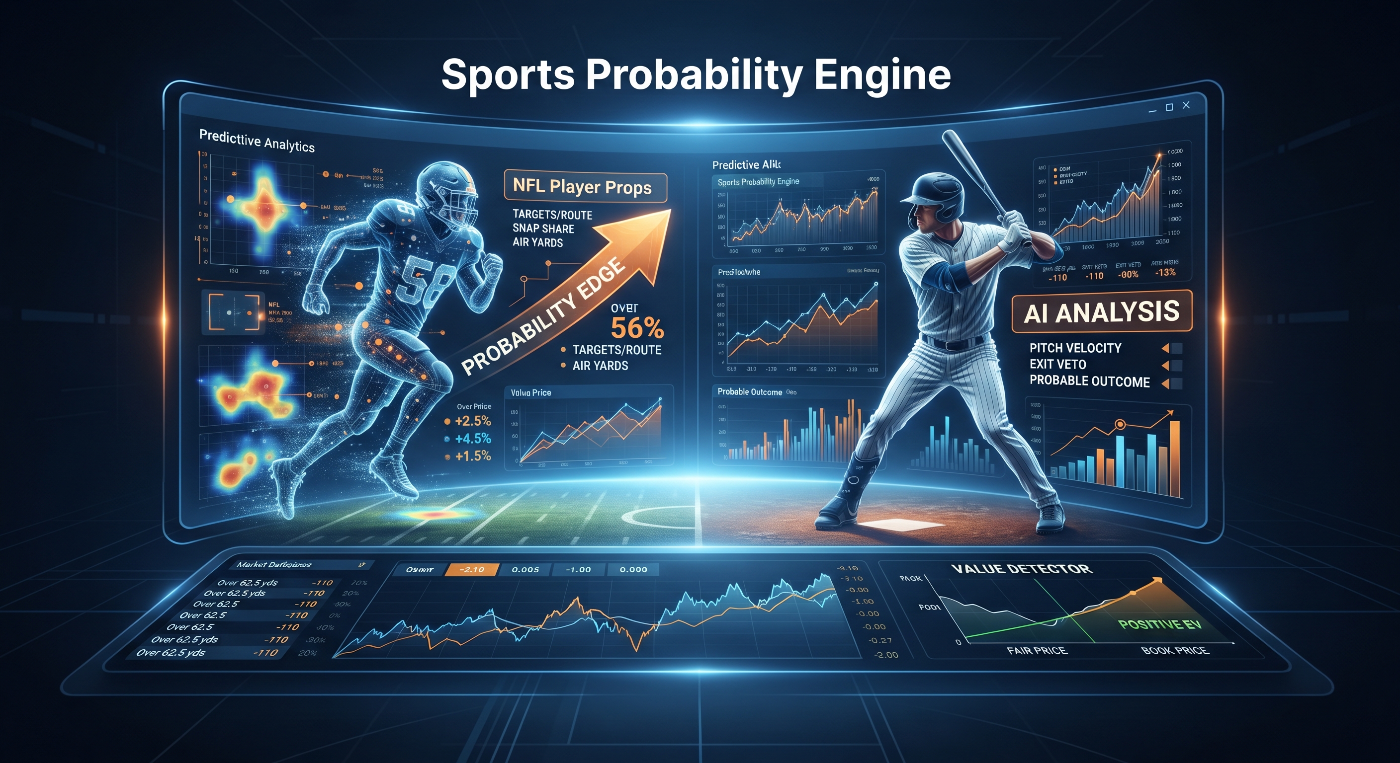
As a pro sports analyst, I will show how I turn raw player tracking, usage trends, and market lines into clear predictions you can act on. We will keep the math friendly, the process transparent, and the results honest by mixing football context with AI models to spot edges, avoid traps, and stay disciplined across a long season. When you look at how modern sports analytics operates, the secret is not just finding a single lucky bet, but building a repeatable engine that processes information faster and more objectively than the general public.
Data inputs and signal quality
What to collect and why it actually moves props
Start with clean, player-level data that maps directly to how books hang numbers. If a feature does not move usage, opportunity, or efficiency, it probably will not move the prop. Snap share and alignment cover total snaps, slot versus wide versus backfield snaps, inline versus slot for tight ends, routes per dropback, and pass-block rate. Usage metrics include targets per route run, air yards, average depth of target, rush share, red-zone carries or targets, and two-minute or hurry-up usage. Team context involves pass rate over expected, neutral-script run and pass tendencies, pace measured in seconds per play, motion usage, and no-huddle frequency. Opponent tendencies incorporate coverage shells, man versus zone rates, blitz and pressure rates, run-box counts, and success allowed to specific roles like wide receiver one versus slot or tight end versus linebacker or safety. Quarterback and offensive line metrics examine time to throw, pressure-to-sack rate, pocket time, and pass-block win rate. Injuries and role signals track practice participation, in or out designations, beat reports, and depth chart movement such as a third wide receiver moving to a second wide receiver role. Weather and stadium details track wind, precipitation, surface type, and dome versus outdoor splits which matter for average depth of target and kicking while still rippling into passing totals. Historical closing lines and closing juice act as priors because the market memory is often the best baseline, especially for volatile players. Use reliable sources such as NFL Next Gen tracking and route context from NFL Next Gen Stats, player logs and splits from Pro-Football-Reference, and play-by-play, expected points added, and derived models from nflfastR. On ATSwins we centralize many of these signals behind the scenes, so bettors can focus on decisions rather than scraping. If you prefer to build, you can still leverage aggregated context while using the ATSwins dashboards to double-check market moves and price drift.
Form priors from historical closing lines
Books tell you what they think. Use historical closing lines and closing vig as a starting distribution per player and prop type. Step one involves collecting the past eight to twenty games of closing lines and final outcomes for each player prop, such as wide receiver receiving yards. Step two computes a rolling implied median from the market after adjusting for juice. Step three regresses your model raw prediction toward this market-based prior with a weight that depends on sample size and player volatility. Step four updates priors weekly and resets weights after role-changing events like an injury return or coaching shift. This stabilizes estimates when samples are small or role signals are noisy.
Handle small samples with Bayesian shrinkage
Small samples make National Football League props tricky, but Bayesian shrinkage helps solve this issue. Empirical priors for a wide receiver with only three games help shrink targets per route run toward positional and team baselines. Partial pooling allows a volatile rookie wide receiver to borrow strength from other rookies in similar roles and overall team passing context. Dynamic weights ensure more snaps and routes reduce shrinkage over time. You can implement this through a practical approach using simple ridge penalties and group means as features to mimic shrinkage, or a full Bayesian approach using hierarchical models that explicitly learn group-level distributions for partial pooling.
Extract, transform, load and sanity checks
You will only be as good as your data, so build a pipeline that is boring and strict. Ingest sources with time-stamped keys including game identifier, play identifier, and player identifier. Normalize team abbreviations, positions, and opponent mappings. Reconcile snap counts versus routes, and if routes exceed snaps, flag and fix the discrepancy. Remove or cap extreme outliers like one hundred percent targets per route run in two-route samples. Confirm injury statuses at ingestion and again sixty to ninety minutes before kickoff. Log data gaps and never silently backfill with zeros. Useful checks include ensuring the sum of team targets equals pass attempts minus throwaways and spikes, air yards sum close to passing yards plus yards after catch allowing for some tracking noise, and player route counts align with team dropbacks when accounting for pass blocking.
Lagged features to prevent lookahead
Do not leak future information into training. Use only lagged statistics from the last three to five games for player opportunity and efficiency. For team metrics like pace and pass rate over expected, use rolling windows that end the prior week. Injury and role changes should encode the expected role for the coming week using practice reports and historical usage rather than final game results. Weather should use forecast windows available at bet time rather than actual post-game weather. A lagging checklist ensures all rate stats are calculated through week minus one, all player status signals are locked at the last news cutoff before kickoff, any opponent splits are built through week minus one only, and no season-end or post-week aggregates are referenced inside pre-week training.
What actually moves props and keeps moving them
Focus on stable drivers that are visible to books but still mispriced in micro ways. Snap share and routes form the backbone of opportunity. Targets per route run and average depth of target provide direct lines to volume and yardage ceilings. Red-zone and two-minute usage account for touchdowns and late receptions which represent earn-it volume. Team pass rate over expected and pace create more plays and more dropbacks which inflate reception and yard props. Opponent pressure changes target depth and quarterback time to throw, shifting wide receiver target mixes. Minor but real edges include early-season uncertainty where roles and rotations shake out and models that shrink smartly win, as well as backup quarterbacks and offensive line injuries where books move the line but the target distribution within a team can swing more than the total.
Templates you will reuse
Data dictionaries require clear column names, units, and update cadence. Weekly data audits use a ten-minute script that flags missing players, route discrepancies, and injury report mismatches. Role-change monitors trigger if snap share delta exceeds fifteen percent or route participation delta exceeds ten percent over the prior three-game average.
Feature engineering and models
Build opportunity features first
Opportunity begets production, so engineer these features with care. Track routes per dropback and route participation rate. Measure targets per route run overall and against man or zone coverage. Follow first-read target share and screen target share. Monitor rush share and design rate distinguishing between designed quarterback runs and scrambles. Track red-zone carries, targets, and inside-the-five usage. Incorporate two-minute drill and third-down participation. Add stability boosts through rolling three, five, and eight game averages with decay giving heavier weight to the most recent games. Calculate z-scores within the team to catch pecking-order changes between wide receiver one and wide receiver two. Apply opponent role filters such as slot wide receiver performance versus slot cornerback target rates.
Efficiency features that do not overfit
Efficiency is noisy, so shrink or cap extremes. Track yards after catch over expected, catch rate over expected by depth bucket, missed tackle rate forced, and contact balance for running backs. Monitor explosive play rate for plays over fifteen yards with a cap at small samples. Evaluate quarterback accuracy and pressure-to-sack rate to contextualize catchable targets.
Game-context signals you will want
Include the Vegas spread and total along with the implied team total. Track team neutral-script tendencies through run and pass splits when win probability is between twenty and eighty percent. Factor in opponent pressure rate and coverage mix for zone versus man rates. Adjust average depth of target deltas for weather by reducing expected depth and completion rate in high winds. Account for pace, no-huddle frequency, and pre-snap motion since these drive marginal play volume.
Model choices for speed and stability
In National Football League player props, you need quick turnaround and robustness. Gradient Boosted Machines like XGBoost or LightGBM handle non-linear tabular signals and interactions quickly. Elastic nets provide fast, interpretable baselines that are hard to break and work well for backstopping and ensembling. Quantile regression estimates medians for median-based lines and upper or lower tails for alternate lines. Hierarchical Bayesian models in PyMC partial-pool volatile players and low-sample roles, making them ideal for rookies and injury-return cases. A practical flow involves training a gradient boosted machine on engineered features for each prop type, fitting an elastic net on a feature subset for a transparent baseline, blending the two out-of-sample, and fitting a PyMC hierarchical model for volatile subsets to yield calibrated medians and uncertainty bands. Apply quantile regression to produce tenth, fiftieth, and ninetieth percentiles for median and alternate line evaluation.
How to do quantile regression for props
Train one model per quantile such as the tenth, fiftieth, and ninetieth percentiles, or use algorithms that natively support quantile loss. Use the fiftieth quantile for a fair median estimate and compare it to the book median line. Use the tenth and ninetieth quantiles to estimate tail hit rates for alternate overs and unders. Calibrate quantiles weekly because miscalibrated tails create fake edges.
Hierarchical PyMC model for volatile players
When roles are not settled, partial pooling matters. Group levels include player, team, position, and week using random intercepts. Key predictors capture opportunity mix including targets per route run and routes, team pass rate over expected, opponent rates, and quarterback or offensive line context. Priors center on positional baselines with wide variance for rookies and low-route players. Outputs generate posterior predictive distributions for yards and receptions with credible intervals. This helps ensure a rookie with two spike weeks does not run away in projections, and a backup thrust into a starting role lands near a positional starter on this team rather than a wild guess.
SHAP for explainability and leakage control
Use SHAP values on your gradient boosted machine to confirm top drivers including routes, targets per route run, pass rate over expected, opponent pressure, spread, and total. Investigate features that look suspiciously predictive like future injury tags or post-game updates. Remove or lag any feature that leaks outcome info such as using final snap shares for the coming week.
Time-based validation that mirrors betting reality
Use time-series splits where you train through week minus one and validate on week t across multiple past seasons. Never mix future weeks into training folds. Score by prop type including receptions, receiving yards, rushing yards, attempts, completions, passing yards, and touchdowns. Track calibration by decile and by role such as starters versus backups or wide receiver one versus wide receiver three. Compare this against random K-fold cross-validation which is fast but leaks time and should be avoided for props, or rolling-origin evaluation which is ideal when performing weekly updates.
A minimal modeling pipeline template
Prepare lagged features and priors including market median and team baseline. Fit an elastic net baseline per prop. Fit a gradient boosted machine per prop and tune with early stopping on time-split validation. Train quantile models at the tenth, fiftieth, and ninetieth percentiles. For volatile groups, fit a PyMC hierarchical model and export the median and eighty percent credible interval. Blend predictions using sixty to eighty percent gradient boosted machine and twenty to forty percent elastic net, overriding with Bayesian medians when uncertainty is high. Save SHAP top features and calibration diagnostics.
Market math and value detection
Turn lines and juice into implied distributions
Lines come with juice that embeds the book margin or vig. For binary props like over or under, convert to implied probabilities. Step one converts moneyline odds to implied probabilities. Step two removes vig by normalizing so over plus under equals one hundred percent. Step three infers a distribution shape for median-based yardage lines using your model quantiles or a parametric fit anchored to the book median if needed. Helpful practices include using your model fiftieth percentile for the fair median compared to the posted number, using tenth and ninetieth percentiles to check if market tails look too fat or thin, and avoiding the assumption of normality since yardage has skew and clumping from game scripts.
Account for correlation across props
Props are not independent of each other. Quarterback and wide receiver stacks mean a wide receiver going over receiving yards correlates with the quarterback going over passing yards. Same-team running back versus wide receiver dynamics mean a run-heavy script depresses wide receiver yards and boosts running back attempts. Same-game dependencies mean spread and total changes alter pass volume symmetrically. Methods to handle this include copulas where you model marginals per player and couple them using historical rank correlations, joint simulation at the game level where you simulate team plays, dropbacks, and target shares before allocating yards to players conditioned on play outcomes, or a quick-and-dirty approach applying correlation penalties when stacking correlated overs and reducing bet size unless joint expected value remains positive.
Simulate outcomes to estimate hit rates
Monte Carlo simulation remains a great tool when books post alternate lines and ladders. Step one samples game context including plays, pace, spread, and total noise. Step two samples team-level pass and run splits conditioned on context. Step three allocates routes and targets from distributions centered on your medians. Step four converts targets to receptions and yards using catch rate over expected and yards after catch over expected draws along with average depth of target dispersion. Step five repeats ten thousand or more iterations to estimate the proportion of outcomes above or below posted lines. Use these simulations to compute hit rates for main lines and alternate ladders, quantify correlation penalties between same-game props, and produce fair prices for same-game parlay combinations while remembering books add hidden margins.
Compute expected value, fair price, and closing line value
Fair price represents the payout implied by your hit rate after removing vig. Expected value per dollar equals the hit rate multiplied by win payout minus the lose rate multiplied by stake. Price thresholds dictate that you only bet when expected value exceeds a preset bar such as plus three to plus five percent after correlation adjustments. Closing line value tracks how often your bet beats the closing line, where persistent positive closing line value is a leading indicator your edge is real. Mispricing persistence measures how often the same player-type edges recur, such as slot wide receivers versus heavy zone teams, and tells you to reduce exposure if the market adapts.
Throttle stakes with fractional Kelly and guardrails
Full Kelly criterion betting is volatile, so use fractional Kelly to survive variance. Step one estimates edge and odds. Step two calculates the Kelly fraction and applies a twenty-five to fifty percent scaling factor for live bankroll management. Step three caps exposure by player, team, and game to avoid correlated drawdowns. Step four uses stop-loss logic to pause if model uncertainty bands widen due to news shocks or if aggregated correlation within a slate is too high. Step five provides late-scratch protection through no-bet options or automatic hedging if inactives surprise players ninety minutes before kickoff. A bet selection checklist asks if the model signal is supported by opportunity features rather than efficiency noise, if vig is removed and fair price is positive after correlation penalties, if simulation confirms your edge at posted numbers, if closing line value trend is positive, if you are within exposure caps, and if you re-checked injury and weather updates.
Practical notes on multi-book shopping
Track multiple books lines and juice because small half-yard differences change expected value. Estimate fair medians first, then choose the book closest to your fair line. Avoid chasing stale numbers if news hits and instead wait for the first equilibrium move unless you have strong conviction in your priors.
Validation and deployment
Backtest weekly and by prop type
Backtest in a way that mirrors your real betting cadence. Train through week minus one and predict week t, scoring hit rate, expected value, and closing line value proxies across prop types including receptions, receiving yards, rushing yards, attempts, completions, passing yards, and touchdowns. Key metrics include calibration curves measuring predicted versus observed frequencies in deciles, Brier scores for binary props, log loss for categorical outcomes, and pinball loss for quantile models. Stability checks measure performance across spread buckets like big favorites versus underdogs, totals from low to high, and weather bins from calm to windy.
Monitor drift when roles change
Markets move faster than models when roles flip. Drift indicators include sudden snap and route share changes, target pecking order shifts where a third receiver leapfrogs a second receiver, and quarterback changes or offensive line injuries altering pass depth and pace. Mitigations involve increasing shrinkage temporarily, reweighting recent games more heavily after a role event, and adding role event binary flags to capture regime shifts.
Alerting: model uncertainty and news ingestion
Set alert thresholds when predictive intervals widen by more than thirty percent week-over-week, when feature importance reorders drastically such as weather jumping to the top driver, or when injury feeds see meaningful status changes from did not practice to limited or full participation. Automate refreshes to rebuild projections every time high-priority news hits, re-run simulations and expected value for impacted players and their teammates, and push hold betting alerts when information is incomplete but relevant.
Maintain experiment logs and post-mortems
Log runs with model version, feature set, training window, validation fold, and data hash. Track changes to see what shifted expected value or calibration. Conduct weekly post-mortems examining the five biggest winners and five biggest losers by expected value, checking whether the signal was opportunity-driven or variance, and seeing if the line moved after you placed your bet. Keep a knowledge base of repeatable edges and dead ends.
Package a lightweight, reproducible pipeline
Stick to standard, well-supported tools that run quickly on slate days. Pandas handles data ingestion, tables, groupbys, merges, and final reports. Scikit-learn manages machine learning workflows, elastic net baselines, pipelines, and time-series splits. PyMC powers Bayesian hierarchical models and posterior predictive checks. Numpy handles vectorized simulation for ten thousand plus runs. Operational shapes remain config-driven with YAML files setting training windows, command-line interfaces for updating data, training, and simulating, caching team and opponent rates per week, and saving flat parquet files with versioned folders for auditability.
Pregame update runbook fast loop
Six hours prior to kickoff involves pulling final practice reports, weather forecasts, and market lines while training and refreshing models. Three hours prior pushes preliminary edges, caps exposure, and sets alerts for questionable players. Ninety minutes prior incorporates inactive announcements, refreshes projections for any changes, and reruns simulations for affected games. Sixty minutes prior represents the bet entry window for line shopping, recording positions, and setting limits. Post-lock logs ticket details and subscribes to live-tracking if you manage in-play hedges.
What we track in production that keeps us honest
Track expected value versus realized efficiency over two to four hundred bets where they should converge. Monitor closing line value by prop type and by book to identify shops you consistently beat. Track model drift using a rolling four-week calibration slope. Attribute edge sources to percentages driven by opportunity versus efficiency versus context. Measure hit rate versus alternative numbers to ensure your edge does not vanish when the line moves half a yard.
How ATSwins operationalizes this work
At ATSwins, our market-aware prior pipelines ingest historical closing lines and juice to set baseline medians per player and prop. Opportunity-first forecasts place routes, targets per route run, red-zone, and two-minute roles at the top of our feature stack, with team pass rate over expected and pace close behind. Bayesian pooling for volatility ensures rookies and role-changers are partially pooled using hierarchical logic so we do not overreact to spikes. Quantile outputs provide every projection with tenth, fiftieth, and ninetieth percentiles to appraise alternate lines properly. Correlation-aware pricing applies copula-style adjustments and joint simulations for same-game props before surfacing edges. Staking and tracking deliver Kelly-fractional staking suggestions, closing line value logging, and persistent edge monitoring to inform bet sizing and stop-losses. Reporting dashboards give at-a-glance views for expected value, closing movement, and model uncertainty to help bettors decide quickly. If you prefer a ready-made setup that implements these pieces with pregame updates and transparent logs, you can explore the ATSwins platform and free resources. Leveraging an advanced nfl player prop edge finder along with comprehensive ai baseball game analysis via a powerful sports probability engine brings professional-grade precision straight to your daily workflow.
References and data tooling adjacent, not competing
NFL route, alignment, and tracking context: NFL Next Gen Stats
Historical player logs and splits: Pro-Football-Reference search player pages and game logs
Play-by-play and expected points added models: nflfastR
Classic machine learning workflows, pipelines, and validation: scikit-learn
Bayesian hierarchical modeling and posterior predictive checks: PyMC
Step-by-step quickstart from zero to a basic edge
1) Assemble and clean week t data
Pull player logs, routes, and snaps through week minus one. Build rolling opportunity features for three and five games. Merge team context including pass rate over expected and pace, opponent tendencies, and weather forecasts. Add historical closing lines for priors.
2) Train fast baselines
Fit an elastic net for each prop and save predictions. Fit a gradient boosted machine for each prop with time-split validation and capture SHAP top features. Train quantile models at tenth, fiftieth, and ninetieth percentiles and inspect calibration.
3) Apply Bayesian stabilization to volatile roles
For rookies, injury-return players, and low-route players, produce a PyMC median and interval. Blend gradient boosted machine and Bayesian medians based on uncertainty.
4) Price the market
Convert book lines and juice to implied probabilities and remove vig. Compare book medians to your fiftieth percentile quantiles. Simulate ten thousand outcomes per game to compute hit rates and fair prices.
5) Adjust for correlation
Penalize stacked overs in the same passing game unless joint simulation confirms the combined expected value. Cap exposure by game and team.
6) Select bets and stake
Set expected value thresholds and filter to top edges. Size with fractional Kelly while respecting per-player and per-game caps. Record lines and times for closing line value tracking.
7) Monitor and react
Re-run after inactives are announced and pull bets if role intelligence flips. Log performance, closing line value, and calibration weekly. Promote repeatable opportunity-driven edges and demote noisy efficiency ones.
Practical patterns that tend to create value
When rushing attempts outpace yardage props
The signal occurs when running back snaps stabilize and the team shifts to run-heavy neutral rates. The edge is that attempts over is often mispriced before yards move because books price yards more reactively. Model tells include rising rush share and positive script projection with modest yards per carry volatility.
Slot wide receivers in high-zone matchups with wind
The signal happens when average depth of target compresses but target volume rises underneath. The edge makes receptions over more attractive than yards with lower tail risk. Model tells include higher zone rates, higher wind speeds, stable quarterback time to throw, and steady slot snap share.
Backup tight end promoted with red-zone packages
The signal appears when total routes are modest but high-leverage usage is present. The edge highlights anytime touchdowns and small reception overs if the line lags the role. Model tells include a spike in inside-the-ten snaps in prior weeks and beat reports hinting at package usage.
Mobile quarterback facing pressure-heavy opponent
The signal occurs when scramble and designed runs increase alongside checkdowns. The edge favors quarterback rush attempts and running back reception overs, while wide receiver deep-yardage unders apply if the line does not adjust. Model tells include defensive blitz rates going up and historically responsive quarterback scramble rates.
Common mistakes to avoid
Data leakage
Using post-game snap shares in pregame features, incorporating final injury statuses unknown at bet time, or blending weeks out of order in cross-validation will destroy your backtests.
Overfitting efficiency noise
Elevating yards after catch or catch rate over expected outliers without shrinkage, or projecting explosive play rates at small samples leads to bad projections.
Ignoring correlation
Stacking multiple overs in the same passing offense without joint simulations or using independent hit-rate math on same-game parlays creates hidden risks.
Betting stale edges
Not line-shopping half-yard differences or failing to move on news when quarterbacks or offensive lines change leaves you exposed.
Minimal artifacts that make you better next week
Weekly calibration reports show decile calibration for each prop type and highlight under or overconfident bands. Expected value attribution pie charts break down edges from opportunity versus efficiency versus context. Closing line value trackers measure average closing difference per prop and per book. Role-change ledgers list players with route or snap deltas exceeding ten percent with annotated reasons. Post-mortem notes provide two bullets on what worked and what failed with links to bets and market moves.
Lightweight tool stack you can run on a laptop
Data and merges rely on pandas. Baselines and quantiles use scikit-learn for elastic nets and gradient boosting with quantile loss. Bayesian stabilization uses PyMC hierarchical models. Simulation uses numpy with vectorized sampling for ten thousand plus runs. Visualization uses simple matplotlib or seaborn calibration and SHAP plots. Scheduling uses cron or a single command-line script with timestamps. Storage relies on flat parquet files with versioned folders for auditability. Keep it boring, deterministic, and documented because the National Football League prop market rewards speed and discipline. The models above, especially when they anchor to opportunity and use the market as a prior, will surface steady mispricings that you can bet with confidence and track with honest metrics.
Conclusion
Artificial intelligence combined with clean roles data, fair odds math, and small-edge staking helps us price props and find value. Stay adaptable and update fast. Try ATSwins, an AI-powered sports prediction platform offering data-driven picks, player props, betting splits, and profit tracking across the National Football League, National Basketball Association, Major League Baseball, National Hockey League, and collegiate sports. Free and paid plans give bettors insights and guides to make smarter, more informed decisions.
Frequently Asked Questions (FAQs)
What does how artificial intelligence finds value in National Football League player props actually mean?
It means using models to spot when a player prop line is mispriced. In short, how artificial intelligence finds value in National Football League player props is by estimating a fair number like a median or hit rate, comparing it to the sportsbook line and price, and flagging positive expected value. If our fair price says over sixty-two and a half yards should be minus one hundred thirty and the market is minus one hundred ten, that represents true value.
Which data matters most for how artificial intelligence finds value in National Football League player props?
The inputs that move the needle are usage and context. For how artificial intelligence finds value in National Football League player props, I look first at role stability including snap share, routes, and targets per route run, along with the game environment featuring pace, spread, and total, plus opponent tendencies. News and injuries matter immensely. Then I fold in pressure rates, coverage types, red zone chances, and weather. Simple truth is that clean roles data beats flashy noise every single time.
How can I apply how artificial intelligence finds value in National Football League player props on game day step by step?
Start with a player role today examining routes, rush share, and two-minute work. Translate that into an honest projection. Compare your fair number to the book line and price, then compute expected value and closing line value. Bet smaller edges, track results, adjust slowly, and never chase losses. This forms the core of how artificial intelligence finds value in National Football League player props, even if you execute it using simple spreadsheets and disciplined personal notes.
How does ATSwins put how artificial intelligence finds value in National Football League player props to work for me?
At ATSwins, we build and maintain artificial intelligence models that highlight when player props are mispriced. ATSwins is an artificial intelligence-powered sports prediction platform offering data-driven picks, player props, betting splits, and profit tracking across major sports leagues including football, basketball, baseball, hockey, and college athletics. Free and paid plans give bettors insights and guides to make smarter, more informed decisions. From my analyst seat, we focus on trustworthy signals, clear probabilities, and easy-to-read dashboards so you can see how artificial intelligence finds value in National Football League player props without any guesswork.
Does price matter in how artificial intelligence finds value in National Football League player props or only the line?
Price matters a tremendous amount. How artificial intelligence finds value in National Football League player props compares both the line and the odds simultaneously. Two overs at sixty-two and a half yards are not the same if one is priced at minus one hundred ten and the other is at minus one hundred thirty-five. If your fair hit rate is fifty-six percent, minus one hundred ten can be positive expected value while minus one hundred thirty-five likely is not. Always check the vig, estimate a fair price, and then make your final betting decision.