Mastering the College Football Player Props Injury Impact Model

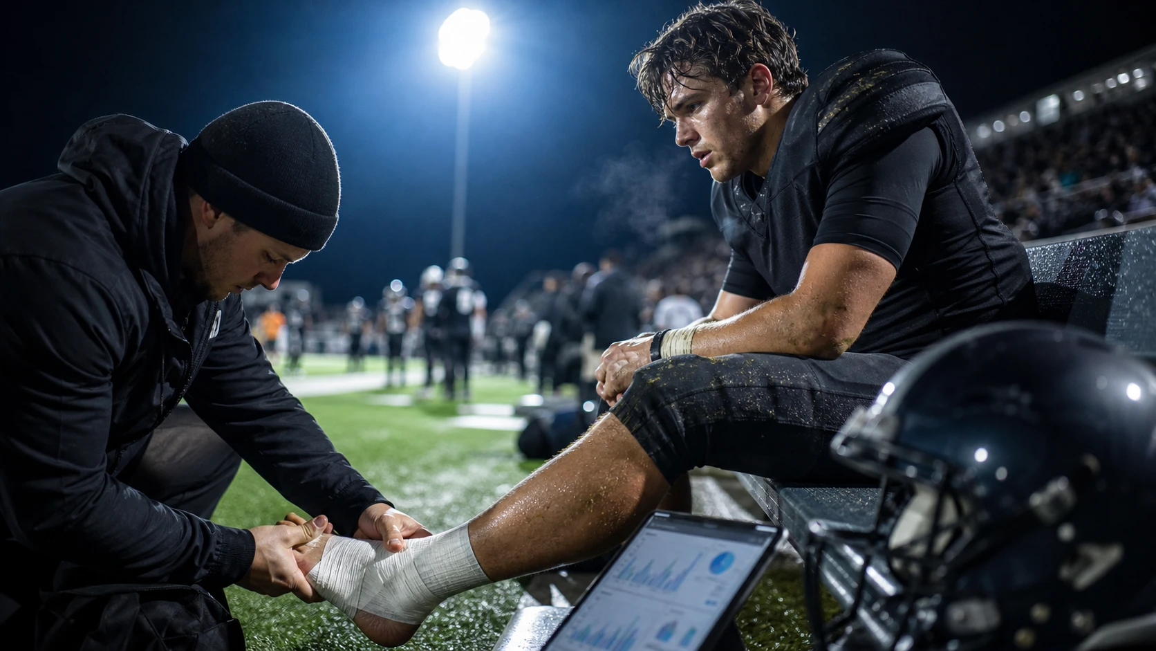
Player props in college football hinge on one thing more than most people realize: injury context and snap share. A player being listed as questionable is not automatically a reason to move a projection down, and a starter being ruled out does not mean every teammate suddenly becomes an automatic over. The real work is figuring out how availability changes playing time, how playing time changes opportunity, and how that opportunity interacts with pace, matchup, game script, weather, and the way a coaching staff actually uses its players.

As a sports analyst who builds AI models, I look at injuries as a chain reaction rather than a single yes-or-no variable. A quarterback injury can change passing volume, sack exposure, scramble expectations, receiver efficiency, and running back usage at the same time. A missing wide receiver can create extra targets for two teammates while also changing the type of routes they run. A running back with an ankle issue might still start but lose goal-line work, explosive runs, or a chunk of his normal snaps. Those details matter when you are projecting pass yards, rush attempts, receptions, and anytime touchdowns.

This is also why injury modeling should not be separated from the rest of the player prop process. The best projection is not simply an injury-adjusted stat line. It is a distribution that tells you what is likely, what is possible, and how much uncertainty is sitting underneath the number. That distinction becomes especially important in college football because rotations, coaching tendencies, quarterback changes, and depth-chart movement can be much less stable than what you might see at the professional level.

Table Of Contents

Key Takeaways

Injuries move college football props by changing snap share first and usage second. A player cannot produce his normal volume if he is not on the field, so availability and snap expectations should be modeled before yards, catches, carries, or touchdown probability. The goal is to set realistic availability odds, apply reasonable snap-limit assumptions, and then translate those changes into the prop markets that are most sensitive to role.

The strongest inputs are clean, time-stamped information about playing time, depth-chart position, recent participation, practice status, team pace, opponent tendencies, and weather. The point is not to collect every possible data point. It is to identify the variables that actually explain opportunity. Route rate, target share, rush share, red-zone usage, neutral-script tendencies, and opponent-adjusted efficiency usually tell you much more than a noisy headline.

The modeling loop can stay relatively simple while still being useful. Injury-adjusted snap and usage models can feed outcome models, while calibration methods help keep the probabilities honest. Backtesting should focus on out-of-sample performance and should measure both projection accuracy and decision quality. When variance becomes too high, passing on a prop is often a better model decision than forcing a pick.

Speed also matters. Injury news can change the entire shape of a slate in a few minutes. When a starter is ruled out, the next player up can move from a minor role into a full-time opportunity, but the exact amount of extra usage depends on the team's substitution patterns. A strong process updates quickly, logs the reason for each change, and later checks whether the assumption was actually correct.

ATSwins can use this framework to turn injury context into a clearer player-prop workflow. The goal is not to pretend that an algorithm knows exactly what will happen. The goal is to give users a transparent projection, explain the major assumptions, show the uncertainty, and help bettors make more informed decisions.

Building a College Football Player Props Injury Impact Model for Smarter ATS Decisions

The foundation of a useful college football player props injury impact model is simple: estimate what a player would do if fully healthy, estimate how likely he is to play and how much he is likely to play, then adjust the expected opportunity around that information. The hard part is making each step realistic.

A common mistake is to start with the injury label and jump directly to the final prop. If a quarterback is questionable, someone might immediately subtract ten passing yards. That approach is too blunt. You first need to ask whether he will play, whether he can handle his normal workload, whether the coaching staff will alter the offense, and whether the backup changes the team's pace or play selection. Only after answering those questions does it make sense to move the passing-yard projection.

The same logic applies to skill players. A questionable running back might have a 70 percent chance of playing, but that does not mean the correct projection is simply 70 percent of his normal rushing attempts. If he plays, he might receive his normal role. If he sits, the carries could be divided among two backs and the quarterback. That creates a mixture of outcomes rather than one smooth projection.

That is why an injury model should be built around distributions. Instead of saying a receiver is projected for 5.2 catches, the model should be able to describe a reasonable middle outcome, a lower outcome, and an upper outcome. The market line can then be compared against that distribution. This is much more useful than relying on a single average that hides uncertainty.

Scope and Goals of a College Football Player Props Injury Impact Model

What we will forecast and the unit of prediction

Four core prop types are especially useful for an injury-driven model: quarterback passing yards, running back rushing attempts, wide receiver receptions, and anytime touchdown scorer. These markets respond quickly to changes in role, and the connection between injury information and opportunity is easier to explain than it is for some of the more specialized props.

For quarterback passing yards, the key question is not just how efficient the passer is. It is how many dropbacks the team is likely to create, how the quarterback's health affects his willingness to throw or scramble, how protection holds up, and whether his receivers can maintain their normal routes. A backup quarterback can change the entire offensive environment even if his raw talent is difficult to quantify.

For running back rushing attempts, volume is usually the starting point. Team plays, expected rush rate, game script, and the player's share of the running-back workload all matter. Injuries become especially important when a committee turns into a two-player rotation or when a quarterback takes on more designed runs.

For wide receiver receptions, route participation is often more important than raw target totals. A receiver cannot earn targets from routes he does not run. Target share, first-read opportunities, quarterback accuracy, average target depth, and opponent coverage tendencies then help translate route participation into catches.

Anytime touchdown props are different because touchdowns are relatively low-frequency events. A player can have a strong role and still fail to score. That means the model should focus heavily on red-zone and goal-line opportunity, team scoring expectation, and the player's share of high-value touches instead of simply using recent touchdown counts.

For each prop, the model should produce a distribution rather than a single number. The median, or P50, gives the central projection. Lower and upper quantiles such as P25 and P75 describe the normal range, while P90 can help identify unusually high-upside situations. The probability of clearing a market line is then derived from the projected distribution.

Why injury information matters most in CFB

College football has a lot of moving pieces. Rotations can be less predictable, freshmen can suddenly earn major roles, coaches can change schemes quickly, and a new quarterback can alter the offense overnight. This makes the injury report more important, but it also makes it easier to overreact.

A quarterback moving from full participation to a limited practice should not automatically be treated as a downgrade of the same size in every situation. The type of injury matters, the timing matters, and the coaching staff's history matters. A player who has regularly practiced in a limited capacity before starting games should receive a different prior than a player who has never dealt with that pattern.

A snap-count limitation is another important example. If a receiver is expected to play but is capped around 50 percent of snaps, the model should not simply reduce his expected catches by 50 percent. His routes could be concentrated in passing situations, his targets could become more valuable, or the team could intentionally use him in specific packages. The relationship between snaps and production is not always linear.

The same idea becomes even more important when a starter is ruled out. The replacement player may receive more snaps, but his efficiency could be lower. The offense might change its play calling. Another player could absorb short-area targets. The quarterback could throw fewer deep passes. In other words, injury impact is a network effect.

The model should therefore treat player availability as a driver of team-level opportunity. When one player leaves the lineup, the system should ask where those snaps, routes, targets, carries, and red-zone touches are likely to go. That reallocation is one of the biggest sources of signal in an injury-aware player-prop model.

On research standards

A strong model does not need to depend on a single source or a single research paper. What matters is that the underlying information is consistent, time-stamped, and validated. Public college football data, official team information, participation reports, practice updates, historical player usage, team statistics, and weather information can all contribute to the model.

Where evidence is limited, conservative assumptions are better than fake precision. If there are only a few games of data for a backup player, the model should shrink his estimate toward a broader team or positional baseline instead of treating a tiny sample as a reliable truth. If a coach's rotation is unclear, the prediction interval should widen.

Data Sources and Ingestion

The data pipeline should begin with play-by-play information, team statistics, player participation, depth charts, practice status, injury updates, opponent tendencies, and game environment. The names of individual websites matter less than the quality and timing of the underlying data.

Play-by-play data is the backbone because it allows the model to calculate how players are actually being used. From each game, the system can estimate team plays, neutral-script pass rate, rushing rate, red-zone behavior, route opportunities, target distribution, and game-script sensitivity. Over multiple weeks, those observations become the player's and team's baseline.

Depth-chart and participation information adds the role layer. A player listed as the second-string running back who played 18 percent of snaps last week should not receive the same replacement projection as a player listed second string who quietly played 45 percent of snaps. Actual participation is usually more informative than a static depth chart.

Practice information should be structured rather than stored as free-form notes. A database can record whether a player was a full participant, limited participant, or absent on each relevant practice day. It can also track whether that status improved or worsened during the week.

Injury information should be time-stamped because old information can be dangerous. A Tuesday estimate should not override a Saturday morning update. The model should know when each piece of information arrived and which projection was built from it.

Weather belongs in the same pipeline because it can change the meaning of an injury adjustment. Wind can reduce the reliability of deep passing and affect quarterback and receiver projections. Rain can influence play calling and ball security. Extreme conditions can increase the value of rushing volume. The exact effect should be estimated from historical data instead of being treated as a universal rule.

Opponent context also matters. A pressure-heavy opponent can make a quarterback injury more meaningful because the backup may hold the ball longer or struggle to create outside structure. A defense that consistently allows efficient rushing can stabilize a running back projection even when the team has some uncertainty around the passing game.

The ingestion process should create a versioned player-week record. Every record should contain the latest known availability status, practice trend, expected snap range, recent role, team context, opponent context, and environment. Keeping historical versions is critical because it lets analysts later answer a very useful question: what did the model actually know at the time the projection was published?

Feature Engineering and Injury Encoding

Raw injury labels are not enough. The model needs to convert them into variables that connect directly to playing time and usage.

A basic availability variable can start with status categories such as out, doubtful, questionable, probable, and available. But status should not be treated as a fixed probability across every team. Coaches have different habits, injury reporting can vary, and certain players are more likely to test pregame than others.

Practice participation adds another layer. A player who misses multiple practices should generally carry more uncertainty than one who progresses from limited to full participation. The important part is to let historical data determine how much each pattern should move the probability rather than assigning arbitrary weights forever.

For skill players, a snap-share prior can be modeled with a probability distribution. A questionable receiver might have one outcome where he plays almost every passing snap and another where he is inactive. If he is active but limited, the model can create a narrower range centered on a reduced snap share. The distribution should reflect the actual behavior of the coaching staff.

Quarterbacks often need a different structure because the outcomes are more discrete. The starter may play zero snaps or nearly all the snaps. A true limited quarterback can be more complicated, but the main model can begin with a mixture of starter and backup scenarios. This makes it easier to capture the huge difference between a healthy starter and a backup running the offense.

Injury type can also influence efficiency. Lower-body injuries may affect rushing explosiveness, route separation, cutting, or scramble ability. Soft-tissue issues can increase the risk of a player being managed during the game. These effects should not be exaggerated, but they can be useful when supported by historical data.

Teammate availability should become part of every player's feature set. If the primary receiver is missing, the secondary receiver's target share can change. If the starting running back is out, the backup's carry share can increase while the quarterback's rushing share may also move. The model should capture those relationships rather than treating each player independently.

Depth-chart deltas are another practical feature. The system can track how many high-usage players are missing from each position group and how much opportunity is available for the remaining players. A receiver-room health index weighted by targets is more useful than a simple count of healthy receivers because losing a 30 percent target-share player is not equivalent to losing a 5 percent target-share player.

Trend breaks need special treatment. When a new quarterback takes over, when a coordinator changes, or when a team dramatically changes its personnel usage, the historical moving average can become misleading. Bayesian shrinkage can help the model blend new information with older data without completely throwing away the past.

Modeling and Validation

The cleanest architecture separates availability, usage, and outcomes. First estimate whether the player will be active and how many snaps he is likely to receive. Then estimate how the team will distribute opportunities. Finally translate those opportunities into the actual prop outcome.

For example, the quarterback layer can estimate expected dropbacks. The usage layer can estimate the team's neutral pass rate and how that rate changes with the quarterback's health. The outcome layer can then estimate completion rate and yards per completion. Passing yards become a product of those linked assumptions rather than a single black-box number.

A tree-based model can be useful for the outcome layer because player props contain nonlinear interactions. A small change in opponent pressure might not matter much for a healthy veteran quarterback but could matter a lot for a backup. The same is true for weather, receiver availability, and game script.

A Bayesian model is useful for the availability and snap-share layers because it naturally represents uncertainty and allows information to be pooled across players, teams, and roles. This is particularly valuable for college football because backup samples are often small.

A practical blended approach is to use Bayesian priors for availability and usage, a flexible tabular model for outcomes, and a calibration step before probabilities are presented to users. The exact algorithms can evolve, but the structure should remain understandable.

Calibration is one of the most important pieces. If a model says a player has a 70 percent chance of hitting a prop, that probability should mean something over a large sample. If 70 percent predictions only hit 58 percent of the time, the model is overconfident even if its average projection looks good.

Distributional accuracy also matters. A model that correctly predicts a median of 70 rushing yards but regularly misses the actual outcome outside its prediction interval is not providing enough information about risk. Metrics such as CRPS and quantile loss can help evaluate whether the forecast distribution is behaving as intended.

For touchdown probabilities, calibration can be measured with Brier score and reliability analysis. A player assigned a 20 percent touchdown probability should score at a rate that approaches 20 percent over a sufficiently large sample of similar predictions.

Backtesting should be chronological. Training on future games and testing on earlier games creates leakage and produces results that look much better than reality. A rolling weekly process is more representative of how the model will actually operate during a season.

Data Transformations, Templates, and Tools

A useful feature dictionary does not need to be enormous. The availability section can include availability probability, expected snap share, practice score, injury type, and expected limitation. Team context can include pace, neutral pass rate, red-zone frequency, and recent play volume.

Player role variables should include route rate, targets per route, first-read share, rush share, short-yardage share, and quarterback scramble rate. Opponent variables can include pressure rate, run-defense efficiency, and coverage tendencies. Environment variables can include wind, precipitation, temperature, and surface.

Recent-form features should be calculated carefully. Three-game rolling averages can help identify current role, but they should be shrunk toward longer-term baselines when the sample is small. A receiver who suddenly runs 95 percent of routes for two games should get a meaningful role adjustment, but the model should not assume that two games completely redefine his talent.

The same concept applies to usage. A backup running back who receives 20 carries in one blowout should not automatically become a bellcow projection. Context has to be attached to every observation.

For an implementation, the data can be organized around a player-week table. Each row represents one player for one game and contains the latest available information before kickoff. That row can include role, team, opponent, practice status, injury information, weather, pace, and recent performance.

The system can also maintain a reallocation configuration by position. If a primary receiver is out, the model can estimate how much of his target opportunity historically flows to the second receiver, slot receiver, tight end, and running backs. If a bellcow running back is out, the system can estimate how often the team uses a two-back committee versus giving the quarterback more designed carries.

The important thing is to treat these values as learned assumptions rather than permanent truths. Reallocation can change when a new offensive coordinator arrives, when a freshman becomes the preferred backup, or when a team changes its personnel groupings.

Practical How-To: Turning Injuries Into Prop Shifts

The first step is to encode availability. Suppose a receiver is listed as questionable and has been limited all week. Instead of saying he is either in or out, assign a probability to each scenario. The exact number should come from historical patterns, but the model could represent one scenario where he is inactive and another where he plays with a reduced role.

The second step is to estimate snap share. If the player is active, ask whether he is likely to run his normal routes or receive a limited package. This is where injury type and practice participation become useful. A player returning from an issue that affects cutting may have a lower route expectation even if he is technically active.

The third step is opportunity reallocation. When a wide receiver is ruled out, do not simply increase every other receiver's projection equally. Look at route overlap, historical target distribution, alignment, and the quarterback's tendencies. The slot receiver might gain short targets while the outside receiver gets more downfield opportunities. A tight end might gain underneath work. A running back might receive more targets as a safety valve.

For a missing bellcow running back, the same process applies. If the team historically uses RB2 on early downs and RB3 in passing situations, the injury should create a split projection. If the quarterback has a strong designed-run role, some of the missing carries may not go to another running back at all.

Quarterback injuries can be even more dramatic. A backup may cause the team to slow down, shorten routes, reduce aggressive throws, or rely more heavily on the running game. The model should make those changes explicitly instead of simply lowering the starter's passing-yard projection.

Opponent and weather adjustments should come after the role adjustment. If the forecast includes strong wind, the passing distribution may become less attractive, but the effect should depend on how the offense normally reacts to weather. A team that already throws short passes may experience a smaller decline than a team that relies heavily on deep shots.

The final step is to convert the adjusted opportunity into a distribution. For a receiver, that can start with routes, targets per route, and catch rate. For a running back, team plays, rush rate, and rush share create the volume estimate. For a quarterback, projected dropbacks and efficiency variables create the passing-yard distribution.

Once the distribution exists, compare it with the market line. If the line sits near the middle of the model's range and the injury uncertainty is high, there may be no reason to take a position. If the model shows a strong probability edge and the underlying assumptions are stable, the prop becomes more interesting.

Case Examples by Prop

Consider a starting quarterback who is questionable and has been limited late in the week. If the model gives him a 55 percent chance of starting, the correct projection is not simply 55 percent of his normal passing yards. The active scenario might produce 260 yards while the inactive scenario might produce 185 team passing yards under the backup. The overall distribution would combine those scenarios, creating more uncertainty than a normal game.

Now consider a bellcow running back who is probable but dealing with an ankle issue. If his healthy baseline is 20 carries, a realistic injury adjustment might center him around a lower workload while preserving some upside. The model should also increase the backup's expected work. If the opponent encourages rushing and the weather supports a ground-heavy plan, the team's overall rushing volume can remain strong even while the starter's individual projection falls.

For a wide receiver, imagine the primary target being ruled out while the slot receiver remains healthy. The slot player's projection should increase, but the type of increase matters. If the replacement receiver is likely to run shorter routes, the catch projection may rise more than the yardage projection. If the outside receiver inherits more downfield routes, his reception median might move only modestly while his upper-tail yardage projection rises.

Anytime touchdown modeling works similarly. Suppose the usual goal-line running back is doubtful. His backup may inherit short-yardage work, but that does not automatically mean the backup has the same touchdown probability. Goal-line packages can include quarterback runs, tight-end concepts, and different personnel groupings. The model should estimate who actually benefits from the missing player's high-value touches.

Validation and Backtesting That Fits Betting Workflows

Backtesting should answer two different questions. First, did the model predict the actual player performance accurately? Second, did the model make better decisions than a simpler baseline when compared with available lines?

The first question is statistical. Track error by prop type, quantify interval coverage, and evaluate calibration. The second question is market-facing. Compare projected probabilities against the price required by the line and track results by confidence level.

It is useful to segment the backtest by injury category. Healthy players should behave differently from questionable players, and snap-limited players should be separated from normal starters. This can reveal whether the injury layer is actually adding signal.

Opponent archetypes can also be useful. A projection against a pressure-heavy defense should be evaluated separately from one against a defense that rarely pressures. The same goes for run-funnel environments and teams that frequently play conservative coverage.

Closing-line movement can provide another diagnostic. If an injury causes the model to move a receiver from 5.5 catches to 7.0 while the market eventually moves from 5.5 to 6.5, the model may be identifying information earlier. That does not prove the model is correct, but repeated patterns like this can show whether its injury adjustments are directionally useful.

SHAP-style feature analysis can also help validate the model. Injury status, snap prior, route rate, rush share, opponent efficiency, and weather should have sensible influence. If an unrelated variable repeatedly dominates the prediction, that is a reason to investigate leakage or overfitting.

The backtest should also track situations where the model correctly decided not to publish a pick. A no-bet decision has value because uncertainty is part of the problem. If a model avoids a large number of unstable game-time decisions and performs better on the cleaner subset, that is a feature, not a failure.

Deployment, Monitoring and Compliance

Before a projection reaches users, the data timestamp should be frozen. The system needs to know exactly what information was available when the prediction was created. Otherwise, analysts can accidentally evaluate a forecast using information that arrived after the line moved.

Late injury news should trigger a targeted recalculation. There is no need to rebuild every player on the slate when one major player is ruled out, but all teammates affected by the injury should be re-evaluated. The system should identify the direct and indirect beneficiaries.

Each model release should have a lightweight model card describing its purpose, target props, data window, major assumptions, calibration results, and known limitations. Versioning matters because injury logic can change during the season.

College football also has unique data challenges. Some opponents provide less granular information, some participation data can be delayed, and small samples can create misleading efficiency numbers. Those limitations should be visible rather than hidden.

API and data-access limits should be respected, and frequently used information should be cached appropriately. The goal is a reliable pipeline rather than a system that depends on repeatedly pulling the same information.

Scheme changes require monitoring too. If a team suddenly changes from a balanced offense to an aggressive passing attack, a four-week moving average may lag behind reality. Large shifts in tempo, personnel, or neutral pass rate should increase model uncertainty until the new identity is supported by enough evidence.

User communication is part of deployment. If a projection moved because a starting receiver was ruled out, the interface should explain that. If weather reduced the upper tail, that should also be visible. Users should be able to understand why the number moved without needing to inspect the underlying model.

How ATSwins Users Can Apply This Model

ATSwins users can apply the framework by treating player props as evolving projections instead of fixed numbers. Early in the week, injury-sensitive players should be flagged for monitoring rather than immediately treated as strong bets. The goal at that stage is to establish a baseline and identify which players could move materially if the news changes.

As practice information arrives, the projection can become more specific. A player who progresses through the week can see his availability probability rise, while a player who remains absent can see uncertainty increase. The important thing is that the projection should change for a reason, not simply because the market moved.

On game day, confirmed inactives become especially valuable because they remove one of the biggest sources of uncertainty. When a primary receiver is officially out, the model can redistribute targets and routes to the remaining players. When a starting running back is out, the team-level rushing projection can be redistributed across the backfield and quarterback.

Weather should be viewed alongside injuries rather than as a separate research task. A quarterback dealing with an issue may already create uncertainty around deep passing, and strong wind can increase the importance of that limitation. A backup quarterback facing difficult weather may also push the offense toward a more conservative plan.

ATSwins can package the result into a projection that includes the median, a reasonable range, the probability of clearing the line, and a short explanation of the injury adjustment. That gives users context without pretending the model has perfect information.

The broader goal of ATSwins is to make sports analysis more useful and easier to act on. An AI-powered sports prediction platform can provide data-driven picks, player props, betting splits, and profit tracking across major sports, including college football. The value comes from putting those pieces together in a workflow where users can see both the projection and the reasoning behind it.

Checklists, Templates, and Quick Wins

A strong pregame process starts with data readiness. Injury and practice information should be current, weather should be updated, depth-chart assumptions should be checked, and opponent context should be refreshed before projections are finalized. If a major piece of information is stale, the model should show more uncertainty rather than quietly treating the old value as current.

A lightweight model card can identify the model version, target props, data window, modeling approach, calibration metrics, and known limitations. It can also record when the model was last updated. This makes it much easier to understand why a projection looked different from the one published the previous week.

The fastest practical improvement is to focus on usage before trying to model every possible efficiency variable. Snap share, route rate, rush share, target share, and red-zone opportunity often provide the strongest connection between injury news and prop outcomes.

Conservative priors are another quick win. If there is not enough information to know whether a backup will receive 35 or 65 percent of the snaps, the model should show a wider range. Precision should come from evidence, not from forcing the algorithm to produce a narrow number.

Quantiles are especially valuable for injury situations because the tails can move much more than the median. A player returning from injury may have a reasonable median but a much lower upper tail if the team is likely to manage his workload. A replacement player may have a modest median but a significantly higher ceiling because of a full-time role.

Soft-tissue injuries deserve careful treatment because they can affect both availability and explosiveness. Again, the goal is not to automatically downgrade every player with the same injury label. It is to learn from historical outcomes and use the evidence to widen uncertainty when appropriate.

Example Scoring Logic for Anytime TD

Anytime touchdown probability can start with the team's expected scoring environment and then move toward the individual player's role. Team scoring expectation creates the overall opportunity pool. Player red-zone share determines how much of that pool belongs to him.

For a running back, carries inside the ten-yard line, goal-to-go usage, and short-yardage participation are more informative than total carries alone. A player with 15 carries but no goal-line role may have a lower touchdown probability than a player with ten carries who consistently handles the highest-value rushing opportunities.

For receivers and tight ends, red-zone targets and end-zone target rates are especially important. The model can also account for motion, alignment, and package usage if enough data exists. A player who only enters on specialized red-zone plays may have a higher touchdown rate per snap than his overall usage would suggest.

Injury status should then scale the player's opportunity. If the player is questionable, the model can blend active and inactive scenarios. If he is active but limited, his red-zone package may not decline as much as his overall route rate. This is exactly why injury modeling should happen at the role level instead of using a blanket percentage reduction.

Opponent red-zone efficiency and expected game script provide the final context. A heavy favorite may create more late rushing opportunities, while an underdog may need more passing touchdowns. The model should use these factors to estimate probability rather than turning them into rigid rules.

Common Pitfalls and How to Avoid Them

One of the easiest mistakes is overreacting to a single injury report. A short practice note can be informative, but it should not automatically produce a dramatic projection shift. Requiring confirmation from participation trends or another credible update can reduce false alarms.

Another mistake is ignoring teammate ripple effects. A missing receiver does not only affect the missing receiver. It changes route distribution, target distribution, protection, quarterback behavior, and sometimes even play selection. The model should account for the entire offensive ecosystem.

Weather is another area where people often overcorrect. Not every windy game becomes a rushing game, and not every rainy game destroys passing efficiency. Teams have different identities and different responses to conditions. Historical team-level behavior should guide the adjustment.

Pace can also be misread. A team's season-long average may not represent the pace it will use in a competitive matchup. Game script, opponent style, and coaching tendencies can all move play volume. A player-prop model should forecast plays rather than blindly importing a season average.

Late news creates a different problem. A model can be statistically strong and still produce a bad user experience if it publishes a confident pick during an unstable injury window. An uncertainty lock can help prevent that. If the player's availability probability remains close to the middle and the possible outcomes are dramatically different, the best action may be to wait.

Finally, do not confuse recent touchdown production with stable touchdown talent. Touchdowns are noisy. Role and opportunity should drive the model more than a player's last two games.

Extending the Model

Once the core markets are working, the same framework can be expanded to longest reception, quarterback rushing yards, and combined rushing and receiving yards. These props often become more interesting when injuries change role or when opponent coverage creates a specific opportunity profile.

Longest reception is especially sensitive to route depth, quarterback aggressiveness, and coverage. An injury can change who runs deep routes, which means a receiver's average targets might remain stable while his probability of recording a long gain changes substantially.

Quarterback rushing yards can benefit from injury modeling because health affects both designed runs and scrambles. A lower-body limitation may reduce rushing efficiency, while a backup quarterback could create more designed rushing plays if the coaching staff wants to simplify the offense.

Combined running back props can also help consolidate uncertainty. If a player is likely to lose rushing work but gain receiving work, a combined market may tell a different story from either individual component.

Data enrichment can eventually include more granular route information, personnel groupings, coverage labels, and in-game snap updates. The closer the model gets to understanding what a player is actually being asked to do, the more useful the injury adjustment becomes.

The key is to add complexity only when it improves out-of-sample performance. More variables do not automatically mean a better model. Every new feature should earn its place through validation.

Compliance, Transparency, and User Value

A transparent projection should clearly separate what is modeled from what is assumed. Snap priors, usage reallocation, weather effects, and opponent adjustments can be modeled from historical data. Some schematic information may still rely on proxies when granular tracking is unavailable.

Users should see uncertainty rather than only a pick. A projection with a narrow interval and stable availability is fundamentally different from a projection built around a 50-50 game-time decision. Presenting those situations in the same way can make the model appear more confident than it really is.

Responsible publishing also means avoiding exaggerated claims. A player prop is a probability problem, not a guarantee. Even a well-calibrated 70 percent projection will lose sometimes. The purpose of the model is to identify situations where the estimated probability and available price appear meaningfully different, while recognizing that variance remains.

Bankroll discipline belongs in the broader user experience too. An edge is not a reason to ignore uncertainty, and a high-confidence model output should not be interpreted as certainty. The system should help users understand risk rather than encouraging them to chase losses or treat every projection as a must-play.

Auditing makes the whole process stronger. Every prediction should be stored with its timestamp, model version, input values, and final result. Analysts can then investigate misses and determine whether the error came from injury news, snap assumptions, usage reallocation, efficiency, or simple game variance.

That feedback loop is what turns an injury model from a one-time project into a useful system. If the model repeatedly underestimates the effect of a missing slot receiver, the reallocation logic can be updated. If weather adjustments are consistently too aggressive, they can be reduced. If backup quarterbacks are producing more rushing volume than expected, that can become a new feature.

Fast-Start Playbook for Analysts

A one-day minimum viable model can start with two seasons of college football play-by-play and roster information. Build basic availability priors from injury status and practice participation. Then create simple models for quarterback passing yards, running back rushing attempts, wide receiver receptions, and anytime touchdowns.

For quarterback passing yards, begin with projected team plays, neutral pass rate, completion rate, yards per completion, and receiver health. For running back attempts, use team plays, rush rate, and expected share. For receptions, use routes, targets per route, and catch rate. For touchdowns, use team scoring expectation and red-zone share.

The next upgrade can introduce a Bayesian snap-share layer and learned reallocation matrices. Add opponent pressure and run-defense variables, weather, and short-week indicators. At that point, dashboards showing calibration and feature influence become useful because analysts can inspect whether the model is behaving logically.

Over a full season, retrain on rolling windows and update priors when coaching or quarterback changes occur. Quantile models can be added once the median projections are stable. The model should become more sophisticated only when each additional layer improves calibration or decision quality.

The most important operational habit is to log every major injury adjustment. If a receiver moves from 5.4 expected catches to 7.1 because WR1 is out, record that reason. Weeks later, analysts can see whether that reallocation assumption was consistently accurate.

What to Surface to Users on ATSwins

A useful player-projection card does not need to overwhelm someone with model internals. The user should see the median projection, a realistic lower and upper range, and the probability of clearing the current line. High-variance props can include a wider range or an explicit uncertainty indicator.

The injury context should be short but meaningful. A note might explain that the player is questionable, has been limited in practice, and carries an expected snap range. If another player is out, the card can explain that additional targets or carries are being reallocated.

A key assumption should also be visible. For example, the model might say that the projection increased because a starting receiver is unavailable and the remaining slot receiver is expected to absorb a larger route share. Another projection might be lower because strong wind reduces the expected passing volume.

There should also be clear situations where the platform does not post a pick. If availability remains deeply uncertain, if a coach has changed the offense without enough new data, or if severe weather arrives immediately before kickoff, the model should be comfortable saying there is not enough confidence.

Tracking is just as important as publishing. ATSwins can evaluate hit rate by injury category, player role, prop type, and uncertainty level. That creates a continuous learning system instead of a static collection of picks.

The overall objective is straightforward. By structuring a college football player props injury impact model around availability, snap share, usage reallocation, opponent context, weather, and calibrated distributions, ATSwins can give users a more complete view of what is driving a projection. The model does not need to predict every game perfectly. It needs to consistently turn relevant information into better estimates and communicate the remaining uncertainty honestly.

Conclusion

Injuries can move college football player props dramatically, but the most useful approach is not to react to headlines. Start with availability, translate that into expected snaps, and then follow the opportunity. From there, layer in team pace, offensive identity, opponent tendencies, weather, game script, and the player's actual role.

The biggest lesson is that injury impact is rarely isolated. A quarterback injury can affect receivers and running backs. A missing receiver can change the distribution of targets across an entire offense. A running back injury can shift carries, pass protection, goal-line work, and quarterback rushing. These are connected outcomes, and the model should treat them that way.

Distributional forecasting is also more useful than a single projection. Median outcomes tell you where the model is centered, but the tails show how much risk is hidden around that number. When an injury creates a wide range of plausible scenarios, that uncertainty should be reflected in the final projection and in the decision to publish or pass.

For ATSwins, this framework creates a practical way to connect injury information with player props, betting splits, projections, and performance tracking. The value is not in promising certainty. It is in giving users a cleaner process for understanding why a number moved, what assumptions are behind it, and when the available information is too unstable to justify a confident position.

The next step is to keep the loop active throughout the week. Establish early baselines, monitor practice participation, update after meaningful injury news, confirm inactive players, and compare the final projection with what actually happened. Over time, those records become a powerful source of information about which injury signals matter most and which ones are mostly noise.

That is the real advantage of an injury-aware player-prop model. It turns scattered updates into a structured decision process. Instead of asking whether an injury is good or bad for a prop, you can ask the better questions: How likely is the player to play? How many snaps will he receive? Where will the missing opportunity go? How does the matchup change that opportunity? What does the distribution look like? And finally, does the market price justify taking the risk?

Frequently Asked Questions

What is a college football player props injury impact model, and why does it matter for betting?

A college football player props injury impact model is a set of statistical rules and predictive models that turns injury information into changes in player-prop projections. Instead of treating an injury as a simple downgrade, the model estimates how availability, snap share, usage, and efficiency are likely to change.

This matters because a player's opportunity is often more important than his raw talent for a single game. If a receiver loses half his routes, his normal per-target efficiency cannot save a reception over if he does not have enough chances. If a running back becomes the clear lead option because the usual starter is out, his projected carries can rise even if his individual efficiency is lower.

The model also helps separate real information from noisy headlines. A questionable designation may mean very different things depending on practice participation, historical coach behavior, injury type, and the player's role. The goal is to price those differences rather than react emotionally.

How do I build a basic college football player props injury impact model to bet smarter?

Start with a small, repeatable system. Collect injury status, practice participation, recent snap share, depth-chart role, team pace, opponent tendencies, and recent usage. Then estimate an availability probability and expected snap range before projecting the actual prop.

Next, reallocate opportunity when a teammate is unavailable. If WR1 is out, identify which remaining players are most likely to absorb routes and targets. If the lead running back is out, estimate how the team divides carries, passing-down work, and goal-line opportunities.

After that, add pace, matchup, weather, and game-script adjustments. Convert projected opportunity into yards, receptions, attempts, or touchdown probability. Finally, compare the resulting distribution with the market line and pass when the uncertainty is too large.

The important part is not making the model complicated on day one. A clean usage model with honest uncertainty can be more valuable than a giant model filled with weak variables.

How do injuries like questionable and snap limits change projections?

Questionable players should usually be represented with more than one scenario. One scenario can represent inactive status, while another represents active status with a normal or reduced workload. The probabilities assigned to those scenarios should depend on practice trends, injury type, and historical behavior.

A snap limit creates a different problem because the player can be active without having a normal role. In that situation, route rate, rush share, designed touches, and red-zone usage can all be reduced. The effect does not necessarily need to be proportional to the snap reduction because coaches can concentrate a limited player's usage in specific packages.

The model should also consider efficiency. Some injuries affect the player's ability to separate, cut, accelerate, or scramble. Those effects can lower the upper tail even when the median does not move dramatically.

What data and updates should I track to keep the model current?

The most important information is current participation, practice status, depth-chart movement, team usage, opponent context, and weather. The data should be time-stamped so the model knows what information was available when each projection was produced.

Updates should happen in stages. Early-week information establishes a prior. Midweek practice participation changes the availability estimate. Late-week updates refine the snap expectation. Game-day inactive news can remove uncertainty and trigger a final reallocation of team opportunity.

The model should not blindly follow market movement either. A line moving can be a useful signal that information has entered the market, but it should be investigated rather than treated as proof that the underlying injury assumption is correct.

How does weather fit into an injury-aware player props model?

Weather can amplify or reduce the effect of an injury. Strong wind can make quarterback and deep-receiver projections more uncertain. Rain can influence play selection and ball security. A team with a limited quarterback may already be inclined toward shorter throws, so weather can reinforce that strategy.

That is why weather should be modeled as part of the same game environment. The article “College Football Player Props Weather Analysis: Smart Wagering Tactics” is a natural companion to this injury framework because both topics are ultimately about identifying how conditions change opportunity and distribution.

The key is to avoid universal weather rules. Historical team behavior, quarterback style, route depth, offensive identity, and opponent tendencies should determine how much a specific forecast moves a prop.

How can ATSwins help with this process?

ATSwins is an AI-powered sports prediction platform designed to bring data-driven picks, player props, betting splits, and profit tracking into one workflow. For college football player props, the value is in having a place to compare projections, monitor changes, and track results instead of treating every prop as a one-off decision.

Users can use injury context to identify players whose projections are likely to move, then monitor how those projections change as practice information and inactive news arrive. Performance tracking can also help users evaluate which types of injury-driven situations have actually been useful over time.

The broader goal is to help bettors make smarter, more informed decisions by giving them context around the number rather than presenting a pick without explanation.

When should a model avoid posting a pick?

The model should avoid publishing a strong position when the availability probability is too uncertain and the possible active and inactive outcomes are dramatically different. A player sitting near a true 50-50 game-time decision can create a distribution so wide that a single market comparison becomes unreliable.

The same applies to major coaching changes, unexpected weather, or unclear depth-chart situations. When the underlying assumptions are unstable, uncertainty should increase.

Passing is not a weakness in a model. It is part of disciplined forecasting. A system that knows when its information is unreliable can be more useful than one that always produces a confident answer.

What is the biggest mistake people make with injury-based player props?

The biggest mistake is usually treating injury news as a direct percentage adjustment to a player's stat line. Football does not work that cleanly. The injury changes snaps, and snaps change opportunity. That opportunity then interacts with play calling, teammates, matchup, weather, and game script.

Another major mistake is forgetting the ripple effect. When one player leaves the lineup, someone else has to occupy those routes, carries, or packages. The best models follow that opportunity through the entire offense.

Finally, people often underestimate uncertainty. A player can be active and still have a completely different role. Modeling that uncertainty is one of the biggest advantages an injury-aware process can provide.

What should a useful ATSwins player-prop projection show?

A useful projection should show the central estimate, a realistic range, the probability of clearing the relevant line, and the most important context behind the number. Injury status, expected snap range, teammate availability, and weather can all be summarized without overwhelming the user.

It should also communicate confidence honestly. A stable projection for a healthy starter is different from a projection built around a questionable player. Users should be able to tell that difference immediately.

Most importantly, the projection should be connected to tracking. Once the game is over, the actual snaps, usage, and result should be compared with the model's assumptions. That feedback is how the system gets better.