

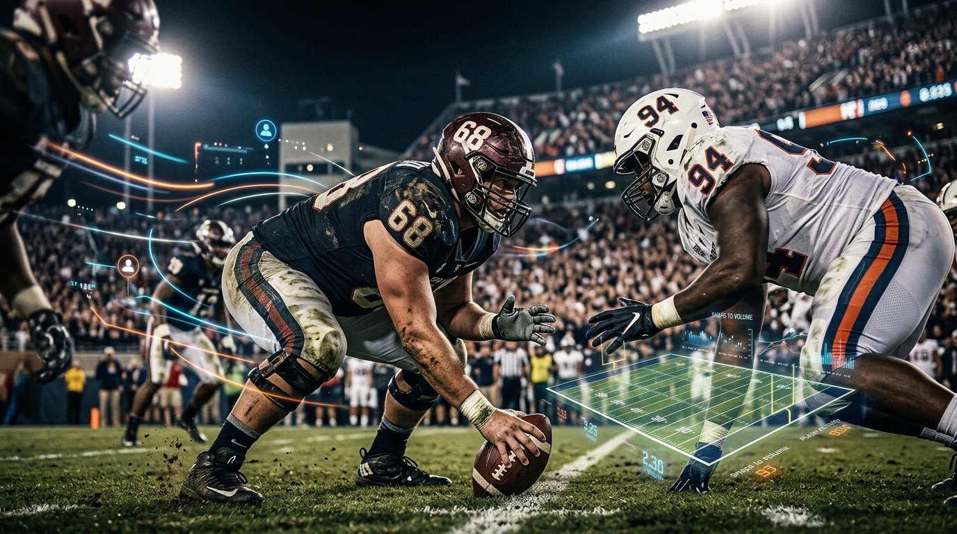
Snap counts are one of the most useful starting points for building college football player props because they tell you something that a normal box score can easily hide: how much a player was actually trusted to play.
A receiver can finish with six catches and 80 yards and look like an obvious target for the next game. But if he only played 55% of the offensive snaps, that production may be harder to repeat. Another receiver might catch only two passes, yet play 90% of the snaps and run routes throughout the entire game. That player could actually have the stronger projection going forward.
That is the basic idea behind college football player props based on snap count. Instead of starting with the final statistics and trying to guess what happens next, start with playing time. From there, estimate routes, carries, targets, and other opportunities before converting those opportunities into a probability for the prop itself.
College football makes this especially interesting because rotations can change quickly. Running backs share work, receivers move in and out depending on formations, tight ends can have completely different responsibilities, and coaches can change personnel based on the opponent. Tempo also changes the number of plays available, while a blowout can remove starters from the field earlier than expected.
The goal is not to predict every snap perfectly. That is unrealistic. The goal is to build a repeatable process that connects playing time to opportunity, opportunity to production, and production to a fair betting price.
Table Of Contents
Why Snap Counts Matter for CFB Player Props
Snap Share vs. Raw Snap Counts
Turning Snaps Into Routes, Carries, and Targets
How Game Script Changes Snap Projections
Building a Reliable Snap Count Baseline
Turning Snap Projections Into Prop Probabilities
Why Matchups Should Adjust the Projection, Not Replace It
Market Timing and Execution
Monitoring Role Changes During the Week
Building an AI-First Snap Count Workflow
Common Mistakes to Avoid
A Practical Weekly Workflow
Conclusion
Frequently Asked Questions
Why Snap Counts Matter for CFB Player Props
When I build a college football player prop projection, one of the first questions I want answered is simple: how much is this player expected to play?
That question sounds basic, but it is easy to overlook when looking at recent box scores. A running back might have 18 carries one week and 10 the next. A receiver might have eight targets in one game and three in another. Looking only at those results can make the player look unpredictable.
Snap counts often explain why.
Raw snaps tell you how many offensive plays a player participated in. Snap share tells you what percentage of the team's offensive plays belonged to that player. For prop modeling, snap share is usually more useful because it lets you compare players across games with different play volumes.
Imagine one team runs 82 offensive plays and another runs 61. A receiver playing 70 snaps for the first team has a different role from a receiver playing 42 snaps for the second team. Raw totals can make those workloads look similar, but snap share gives you the context.
A player consistently playing 85% to 90% of offensive snaps has a fundamentally different projection from someone sitting around 45% to 55%. Even if both players produced similar statistics last week, the high-snap player usually has a stronger opportunity foundation.
This matters even more in college football because rotations can be aggressive. A team may have three talented running backs, four receivers who all see legitimate playing time, and multiple tight ends who are used differently depending on the formation. Being listed as a starter does not necessarily mean a player has a full-time role.
That is where snap analysis becomes useful.
For wide receivers and tight ends, snaps create opportunities to run routes. Routes create opportunities for targets. Targets create opportunities for receptions and receiving yards. The chain is not guaranteed, but it gives you a logical structure for the projection.
For running backs, snaps create opportunities for carries and targets. But not every running-back snap has the same value. A third-down back might play fewer total snaps while running more routes. A short-yardage back might see fewer passing opportunities but receive a larger share of goal-line carries.
Quarterbacks are different because they normally play nearly every offensive snap. Their snap count is less useful as a differentiator, so the focus shifts to what happens on those snaps. Designed runs, scrambles, sacks, dropbacks, and game script become more important.
That is why snap count is the foundation, not the final answer.
Snap Share vs. Raw Snap Counts
Raw snaps are straightforward. If an offense runs 70 plays and a receiver participates in 63, that receiver played 63 offensive snaps.
Snap share takes that number and divides it by the team's total offensive snaps. In this example, the receiver played 90% of the offensive snaps.
That 90% tells you something important about the player's role.
Now imagine another receiver plays 42 snaps in a game where his team runs 60 plays. His raw snap count is lower, but his snap share is 70%. If that team normally plays at a slower tempo, that can still represent a meaningful role.
This is why I prefer projecting team play volume and player snap share separately. First estimate how many plays the team is likely to run. Then estimate what percentage of those plays belong to the player.
College football also creates situations where raw snap counts can be misleading. A heavily favored team may use starters for most of the first half and then rotate younger players once the result is basically decided. Those backup snaps still appear in the final numbers, but they do not necessarily represent a new permanent rotation.
The opposite can happen in a close game. A coach may rely on a smaller group of trusted players, pushing a starter's snap share higher than normal.
Game script therefore needs to be part of the analysis.
I like thinking about snap share as a measurement of role rather than simply a measurement of volume. A player consistently playing 85% of snaps is telling you that the coaching staff trusts him in multiple situations. He may play early downs, third downs, two-minute situations, red-zone possessions, and obvious passing situations.
A player at 45% may have a more specialized role. That does not automatically make him a bad prop target. It just means you need to understand why he is playing those snaps.
For example, a receiver playing only 60% of snaps could still have a strong reception projection if most of his snaps come in passing formations and he is the primary slot option. Meanwhile, a receiver playing 80% of snaps could have a weaker target projection if a large portion of those snaps involve blocking.
The real question is not simply how many snaps a player gets.
The real question is what he does when he is on the field.
Turning Snaps Into Routes, Carries, and Targets
Once I have a projected snap share, the next step is translating those snaps into actual opportunities.
For receivers, routes are the bridge between snaps and targets. A receiver needs to be running a route before a normal passing target can occur. That makes route volume one of the most useful follow-up measurements.
Suppose a team is projected to run 76 offensive plays and pass on 52% of them. That gives us roughly 40 expected dropbacks. If a receiver is projected to participate on 90% of the relevant passing snaps and runs a route on 95% of those opportunities, the initial route projection lands around the mid-30s.
From there, target rate becomes important.
If the receiver earns targets on about 21% of his routes, the initial projection might land around eight targets. Catch rate can then be applied to estimate receptions, while target depth and receiving efficiency help shape the receiving-yard projection.
Notice how much more information this gives you than simply saying that the receiver averaged seven targets over the last three games.
The snap-based approach explains where those targets are expected to come from.
The same concept works for running backs.
Suppose a team is expected to run 44 times. If the lead back owns about 65% of the rushing workload, the first projection is around 29 carries. But that number still needs adjustments. If the team is a major favorite, the back may receive more carries late. If the team is expected to trail, passing-down work could shift toward another back.
A running back's role can also be split by situation. First and second downs, third downs, two-minute drills, red-zone possessions, and short-yardage plays can all use different personnel.
This is why two backs with identical snap shares can have completely different prop profiles.
The same issue appears with tight ends. One tight end might play 70% of snaps but run routes on only half of them. Another could play 55% while running routes on nearly every passing snap. If the prop is receptions, the second player might have the stronger opportunity profile.
Quarterback rushing props require another layer. Designed rushing attempts, scramble rate, pressure, and game script all matter. A quarterback who averages four designed runs per game does not automatically become a strong rushing-over candidate because the opponent has allowed rushing production to quarterbacks.
But if that opponent creates pressure and uses man coverage frequently, scramble opportunities can rise. If the quarterback also has a consistent designed-run package, the combination can create a meaningful increase in expected rushing volume.
How Game Script Changes Snap Projections
One of the easiest ways to make a snap-based projection better is to stop treating every game as if it will follow the same script.
A favorite and an underdog can have very different usage patterns even when their players have identical season averages.
Consider a team favored by several touchdowns. The starting running back might normally play 70% of the snaps, but the projection should not blindly assume that number. If the team is likely to build a large lead, the coaching staff may rotate the second and third backs during the second half.
That can reduce rushing attempts for the starter even if his first-half role is excellent.
The opposite situation can create more passing volume. An underdog expected to trail may run fewer total plays but throw at a higher rate. That can increase the opportunity for its primary receiver even if the team is not expected to score many points.
This is why I separate total snaps from role.
A team can run 80 plays and still give a receiver fewer opportunities than expected if the offense uses heavy personnel. Another team can run 68 plays while funneling a large share of passing opportunities toward one receiver.
The expected game script should influence the distribution rather than simply changing one number.
Blowout risk also needs to be handled carefully. Garbage-time production is real production, but it does not always represent a player's normal role. If a backup receiver gets 15 snaps in the fourth quarter because the starters were removed, those snaps should not automatically be treated as evidence that his role has expanded.
The same principle applies to running backs.
If the starter receives 20 carries before halftime and the backup receives 12 carries after the game is out of reach, the final box score may make the rotation look much more balanced than it really was.
For prop modeling, I want to know when those opportunities occurred and why.
Building a Reliable Snap Count Baseline
If you want to consistently build college football player props based on snap count, you need historical context.
A single game is not enough.
I prefer keeping rolling measurements for snap share, route participation, target rate, carry share, targets, and rushing opportunities. Three-game and five-game windows are useful because they balance recent information with stability.
The latest game should not automatically receive the most weight.
Imagine a receiver who plays 91%, 90%, and 88% of snaps before dropping to 65% in the next game. If that fourth game was a massive blowout, I would not suddenly assume his role collapsed.
But if he played 65% in a competitive game and the coaching staff openly discussed a rotation, that is different.
Context determines whether the change is signal or noise.
I also like assigning internal role labels. These can be simple. A player might be treated as a full-time receiver, rotational receiver, slot specialist, blocking tight end, passing-down back, short-yardage back, or goal-line back.
The labels help prevent the model from treating every snap as equal.
Another useful measurement is snap volatility.
If a player's snap share moves only a few percentage points from week to week, the role is probably stable. If it regularly moves by 15 to 25 percentage points, the projection should be wider.
That does not automatically make the player a bad bet. It means the price needs to compensate for the uncertainty.
Averages can hide this problem.
A receiver with snap shares of 50%, 90%, 50%, and 90% has an average of 70%. But projecting him for exactly 70% every week would be misleading. His actual role is much more volatile.
That can dramatically change the probability of an over or under.
Turning Snap Projections Into Prop Probabilities
This is where the process becomes a real betting model.
I start with the team projection. How many offensive plays should the team run? What percentage should be passes? What percentage should be runs?
Those numbers create the opportunity pool.
Suppose a team is projected for 78 plays and a 51% pass rate. That produces roughly 40 expected dropbacks. If the lead receiver is expected to run routes on 92% of those passing opportunities, the initial route projection is around 37.
Then I estimate target rate.
If the receiver has a 21% target-per-route rate, the expected target count is around eight. From there, catch rate gives me a starting reception projection.
But I do not want to stop at the expected value.
The real question is how often the receiver reaches four, five, six, seven, or more catches.
That requires a distribution.
For receptions, target volume can be modeled from route volume and target rate, followed by a catch-rate assumption. For rushing attempts, team rushing volume can be combined with carry share. Yardage requires more variance because explosive plays can create heavily skewed results.
This is especially important for receiving yards.
A receiver can have eight targets and finish with 45 yards or 140 yards depending on target depth and one or two explosive plays. Simply multiplying expected receptions by last week's yards per catch can hide that uncertainty.
Longest-reception props are even more volatile.
A receiver can have a strong overall receiving projection while still being a poor candidate for a longest-reception over if he rarely receives downfield targets. Conversely, a player with modest expected reception volume can have serious longest-reception upside if his route tree consistently creates deep opportunities.
Once I have the simulated distribution, I can compare it with the betting line.
If a model gives a player a 58% probability of going over 4.5 receptions, that can be converted into a fair price. If the market offers a meaningfully better price, the wager may have value. If the market has already moved close to the model's fair number, there may be no reason to force the bet.
That is one of the most important lessons in prop betting: a good projection does not automatically create a good wager.
Why Matchups Should Adjust the Projection, Not Replace It
Snap counts provide the foundation, but matchup information can improve the final projection.
The mistake is treating matchup statistics as a replacement for role analysis.
If a defense has struggled against wide receivers, that does not mean every receiver on the opposing team deserves an over. You still need to know who is playing and how the team distributes routes.
The same applies to running backs. A strong run defense may reduce expected yards per carry, but it does not necessarily make a rushing-attempt under attractive if the back is expected to receive a large workload.
I like separating volume from efficiency.
Pressure is another useful variable. A high-pressure defense can reduce the time available for deep routes while encouraging quick throws. That may help short-area receivers and tight ends while reducing the probability of a long completion.
Coverage structure can also influence target distribution. Two-high looks can push offenses toward underneath targets, while single-high structures can create more opportunities for boundary receivers to attack vertically.
Box counts matter for running backs because defensive alignment can influence rushing efficiency. A light box can improve the environment for explosive runs, while a heavy box can make rushing efficiency harder.
But these should be adjustments rather than absolute rules.
If the coaching staff has repeatedly shown that it will feed the same running back regardless of the defensive front, the player's volume may remain strong even when the efficiency projection falls.
That is why I prefer modest matchup adjustments. The player's role should usually remain the main driver, while the matchup shapes the range around that role.
Market Timing and Execution
Having the right projection is only half the job.
You also need the right number.
College football props can move quickly when meaningful role information becomes available. If a starting receiver is ruled out, the market can immediately change expectations for the remaining receivers. If a running back is limited close to kickoff, carry and target projections can move within minutes.
This is where snap research becomes especially useful.
If you already understand how the team's rotation works, you can react faster than someone who is only looking at the box score.
Suppose a team normally rotates three receivers but the third receiver becomes unavailable. The obvious reaction may be to increase the top receiver's targets. But the more important question is how the coaching staff handled similar situations previously.
Did the second receiver move into a full-time role? Did the tight end absorb more routes? Did the team change its personnel groupings?
Historical snap information can help answer those questions.
The same applies to running backs. If RB2 is unavailable, it does not automatically mean RB1 receives every remaining carry. The team could promote another player, increase quarterback rushing, or use more passing plays.
The market may price the obvious replacement too aggressively.
Timing also means knowing when not to bet.
If your projection depends on incomplete injury information, waiting can be better than forcing an early position. If the role is clear and the market has not adjusted, early entry may offer the better number.
I also recommend tracking closing-line movement. A bet that loses does not automatically mean the process was bad. If you consistently beat the closing price, that is evidence that your timing and pricing process may be working even when short-term variance goes against you.
ATSwins can help with this part of the process by bringing player prop projections, market information, betting splits, and performance tracking into the same workflow. Its player-prop tools provide AI-driven projections and confidence grades, giving bettors another reference point when comparing their own assumptions with available markets.
Building an AI-First Snap Count Workflow
AI can make this process faster and more consistent, but it should not replace football logic.
I think about the workflow in three layers.
The first layer is team context. The model estimates offensive plays, pace, pass rate, rushing rate, expected game script, and other team-level variables.
The second layer is player role. The model estimates snap share, route participation, carry share, target rate, and other workload measurements.
The third layer converts those estimates into probabilities for individual props.
This structure is important because it stops the model from jumping directly from historical box scores to a betting line.
For example, if a receiver's historical average is 5.5 catches but his expected route volume has increased because his snap share has become more stable, the model has a reason to increase the projection.
If his snap share falls because another player has earned a larger role, the model has a reason to lower it.
AI is particularly useful for identifying patterns across large samples. It can find situations where certain players gain snaps when teammates are inactive, where a team changes its rotation against specific personnel groups, or where game script consistently changes running-back usage.
But human judgment still matters.
Coaches can change plans. Young players can suddenly earn more work. Transfers can change an offense. A coordinator can introduce a new package that was not present in the previous season.
That is why I prefer a hybrid process.
Use historical data and AI to create the baseline, then use current information to adjust the role assumptions.
ATSwins fits into that workflow because it provides AI-based sports projections, player props, betting splits, and tracking across NCAA and other major sports. The platform is designed to help bettors compare data-driven signals with market prices and review performance rather than relying only on memory.
Common Mistakes to Avoid
One of the biggest mistakes is confusing participation with meaningful offensive usage.
A player can technically appear in a game without having a stable role. If every appearance is treated as evidence of a full workload, the projection can become inflated.
Another mistake is overreacting to one game.
A receiver moving from 55% to 90% of snaps is interesting, but you need to know why it happened. If the increase came during a blowout, the signal may be weaker. If it happened in a competitive game and route volume also increased, the signal is much stronger.
Another common mistake is ignoring game script.
A heavy favorite may have a strong offensive projection but fewer fourth-quarter snaps for its starters. An underdog may throw frequently but struggle to sustain drives.
Quarterback rushing props have their own trap. A quarterback can have strong scrambling ability but still miss a rushing-yard line if the opponent creates consistent pressure and sacks him. Designed rushing volume, scramble rate, and sack risk all need to be considered together.
I also avoid treating recent efficiency as permanent.
A running back averaging 7.5 yards per carry over two games may have benefited from several explosive plays. A receiver averaging 20 yards per catch may not receive the same target depth next week.
Opportunity is generally more stable than short-term efficiency.
Finally, do not chase a number after the market has already moved past your edge. If you liked an over at one price and the line moved significantly, your original reasoning may still be correct while the current wager becomes unattractive.
Being right about the player does not mean the current price is right.
A Practical Weekly Workflow
I like starting the week by reviewing the previous game's snap distribution.
The goal is not simply to record the numbers. I want to identify role changes. Which receiver became a full-time player? Which running back lost third-down work? Did a tight end suddenly run more routes? Did a quarterback receive additional designed rushing opportunities?
After that, I establish initial team projections.
I estimate offensive play volume, pass rate, rushing rate, and likely game script. These numbers create the foundation for the player-level projections.
Next, I convert team assumptions into individual opportunities.
For receivers, that means routes, targets, receptions, and receiving yards. For running backs, it means snaps, carries, targets, and rushing yards. For quarterbacks, it means dropbacks, attempts, designed runs, scrambles, and potential sack exposure.
Then I apply matchup adjustments.
I look at pressure, defensive structure, expected box counts, pace, and game environment. I do not want one matchup statistic to dominate the model. Each variable should make a controlled adjustment.
By the middle of the week, I start thinking about prices.
For every prop, I want to know my estimated probability and the price that would make the wager worthwhile. That gives me a target number instead of encouraging me to bet simply because I like the player.
As kickoff approaches, I monitor role information.
If a player is trending toward a larger or smaller snap share, the projection needs to move. If the information is unclear, uncertainty should increase rather than being hidden.
Before kickoff, I make one final review of the expected personnel and role assumptions.
After the game, I record the results and compare them with the original projection.
If I projected 85% snap share and the player received 62%, I need to understand why. If the player received 86% and still missed the prop, that is a different outcome. The first may indicate a role-model problem. The second may simply be normal variance.
That distinction is essential for improving over time.
Conclusion
College football player props based on snap count are really about understanding opportunity before trying to predict the final stat line.
The process starts with expected playing time. From there, you estimate routes, carries, targets, and other opportunities. Then you layer in team pace, pass rate, game script, matchup conditions, injuries, weather, and role changes. The important thing is to keep the order logical. Do not start with a yardage number and work backward. Start with the player's expected role and build the projection from there.
Snap share should also never be treated as an isolated statistic. A receiver playing 85% of snaps is more interesting when those snaps turn into a high route rate. A running back's 70% snap share means more when he also owns early-down, passing-down, and goal-line work. A quarterback's nearly full-time snap share becomes useful when you understand how many designed runs and scramble opportunities exist within those plays.
The goal is not to predict every game perfectly. Variance is unavoidable, and even a strong role projection can lose when a player misses a target, a runner gets tackled at the goal line, or an explosive play goes the other way. Good modeling is about making better probability estimates and comparing those estimates with the price available in the market.
This is also where tracking matters. ATSwins can complement a snap-count workflow by providing AI-driven player-prop projections, confidence grades, betting information, and performance tracking. Its player-prop tools are designed to surface data-driven projections when odds are available, which gives you another reference point for comparing your own research with the market.
The most useful approach is simple: understand the role, project the snaps, convert those snaps into opportunities, build a range of outcomes, compare that range with the market, and stay disciplined when the price no longer makes sense.
College football has a huge number of moving parts, but snap counts provide one of the clearest ways to connect what happens on the field to what happens in the player-prop market.
Frequently Asked Questions
What does college football player props based on snap count mean?
It means starting a player-prop projection with expected playing time instead of starting with final box-score statistics. For a receiver, expected snaps can be converted into routes, routes into targets, and targets into receptions and receiving yards. For a running back, snaps can be converted into carry share and target opportunities. For quarterbacks, the focus can shift toward dropbacks, designed rushing opportunities, scrambles, and sacks. The basic idea is simple: players need opportunities before they can produce statistics.
Why is snap share more useful than raw snaps?
Snap share puts playing time into context. A player who records 60 snaps in a 75-play game played 80% of his team's offensive snaps. Another player with 60 snaps in a 90-play game played only 67%.
Both have the same raw total, but their roles are different. Snap share also makes it easier to compare players across teams with different offensive tempos.
How do I turn snap share into a college football player prop?
Start by projecting team offensive plays and the expected pass and run rates. For a receiver, estimate route participation and target rate, then apply catch rate and expected target depth. For a running back, estimate team rushing volume and the player's carry share while separating passing-down work.
For a quarterback, estimate dropbacks, designed runs, scramble opportunities, and sack exposure. Finally, turn those assumptions into a probability distribution instead of relying on one point projection.
Should I use one game's snap count?
Usually, no.
One game can be affected by injuries, blowouts, unusual personnel packages, or unexpected game script. A rolling sample of several games provides a stronger baseline.
However, recent games deserve more attention when there is clear evidence of a real role change. A receiver moving from roughly 55% snap share to more than 80% over several competitive games is much stronger evidence of a new role than one isolated spike.
How does ATSwins fit into this process?
ATSwins is an AI-powered sports prediction platform that provides data-driven insights including player props, betting splits, and performance tracking. Its player-prop tools provide AI-driven projections and confidence grades, which can be used alongside your own snap-count research when comparing player expectations with available market prices.
The important part is still the process. Snap information, role analysis, matchup context, probability estimates, and price all need to work together.
ATSwins can complement that workflow by helping you organize the research, review available projections, and track how your decisions perform over time.