

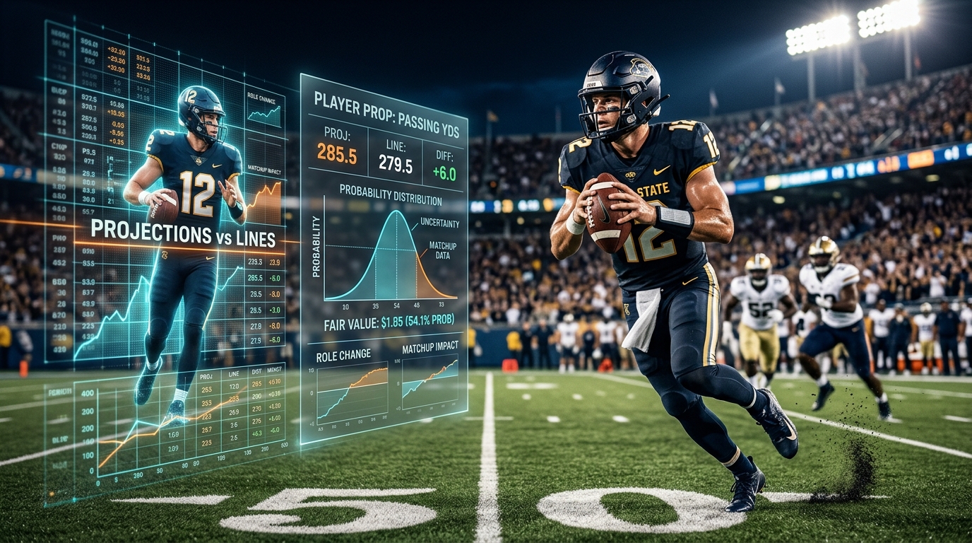
A college football player prop projection vs sportsbook line comparison is essentially a test of two numbers: what a statistical model expects a player to produce and what the market is asking you to predict.
If a model projects a quarterback for 286 passing yards while a sportsbook posts 261.5, the 24.5-yard difference looks interesting. But the gap alone does not establish value. A useful comparison also considers the player's expected workload, opponent, game environment, injury news, weather, distribution of possible outcomes, and how confident the model is in its estimate.
That distinction matters because a projection is not a guarantee and a sportsbook line is not necessarily a prediction of the player's exact result. The line is a threshold attached to an outcome. The goal of serious analysis is to determine whether the probability implied by that line differs meaningfully from the model's estimated probability.
This article explains how to compare a college football player projection with a sportsbook prop line without treating a raw projection difference as an automatic betting signal.
Table of Contents
Projection vs. Sportsbook Line: What Are You Comparing?
How a College Football Player Projection Is Built
How to Measure the Projection Gap
Why Probability Matters More Than the Raw Difference
What Can Move a Player Projection?
A Practical College Football Prop Example
How ATSwins Fits Into the Process
Turning Projection Differences Into Better Analysis
Frequently Asked Questions
- Projection vs. Sportsbook Line: What Are You Comparing?
- The simplest version of the comparison is straightforward.
- Suppose a model projects a running back for 94 rushing yards and a sportsbook posts an over/under of 81.5 yards. The projection is 12.5 yards higher than the line.
That is useful information, but it is only the beginning.
A projection represents an estimate of expected production. A sportsbook prop line represents a threshold. The two numbers answer different questions. The projection asks, "What does the model expect this player to produce?" The prop asks, "Will the player finish above or below this number?"
Those questions become connected when the projection is converted into an outcome distribution.
For example, a model might project 94 rushing yards but estimate substantial variance because the player could receive anywhere from 12 to 25 carries depending on game script. Another player might also project for 94 yards but have a much tighter expected workload.
The identical projections do not necessarily produce identical over probabilities.
That is why the most useful college football player prop analysis moves beyond comparing one number with another.
How a College Football Player Projection Is Built
A serious player projection begins with a collection of inputs rather than a single season average.
Official NCAA statistics provide individual measures such as passing yards, rushing yards, receptions, touchdowns, yards per carry, and other player-level statistics.
More granular college football datasets can add game-level information, play-by-play data, player usage, advanced metrics, weather, and historical betting lines. College Football Data, for example, provides access to player statistics, play-by-play information, weather, advanced metrics, and betting data.
A player projection can then incorporate factors such as recent workload, season-long production, opponent quality, offensive pace, expected plays, team scoring environment, receiving or rushing opportunity, and player role.
The important word is expected.
A running back averaging 5.8 yards per carry does not automatically receive a projection based on 5.8 multiplied by an assumed number of attempts. A model also has to estimate whether the player will actually receive those attempts and whether the matchup changes his expected efficiency.
The same applies to quarterbacks and receivers.
A quarterback's passing-yard projection can depend on expected dropbacks, completion rate, yards per attempt, opponent pressure, game script, and other variables.
A wide receiver's receiving projection can depend heavily on target opportunity, route participation, quarterback tendencies, defensive matchup, and expected pass volume.
This is where a model becomes more useful than a simple recent-game average.
How to Measure the Projection Gap
The first calculation is simple:
Projection Gap = Model Projection − Sportsbook Line
Imagine the model projects 72.0 receiving yards and the sportsbook line is 61.5.
The raw gap is:
72.0 − 61.5 = +10.5 yards
A positive number means the projection is above the line. A negative number means the projection is below it.
But the size of the gap should be interpreted relative to the player's normal variance.
A 10.5-yard gap might be significant for a receiver with a narrow distribution of expected outcomes. It may be much less meaningful for a boom-or-bust deep threat whose receiving yardage regularly swings by 50 or more yards from game to game.
This is one reason standardized differences can be useful.
A simple analytical framework can compare the projection gap with the model's estimated standard deviation:
Projection Difference ÷ Projected Standard Deviation
If a receiver has a 10-yard projection gap but a 35-yard estimated standard deviation, the difference is relatively modest.
If another player has the same 10-yard gap with a 15-yard standard deviation, the separation is much larger relative to the expected range of outcomes.
This does not automatically create a betting recommendation. It simply gives the raw difference more statistical context.
Why Probability Matters More Than the Raw Difference
The central mistake in comparing a college football player prop projection with a sportsbook line is assuming that the projection itself tells you whether the over or under is attractive.
It does not.
Suppose a model projects a receiver for 84 yards and the sportsbook line is 74.5. The projection is 9.5 yards higher.
To evaluate the over, the model needs to estimate the probability that the receiver actually exceeds 74.5 yards.
That requires a distribution rather than just a mean.
For illustration, assume a hypothetical model produces an estimated 61% probability of the receiver going over 74.5 yards. If the sportsbook's price implies a materially lower probability after accounting for the odds and vig, the comparison becomes more interesting.
This distinction is central to sports modeling.
A projection of 84 yards does not mean the player will get 84 yards. It means 84 is the model's estimate of the expected outcome.
A well-calibrated model should also be evaluated over many observations. If forecasts labeled around 60% probability actually occur approximately 60% of the time over a sufficiently large sample, that provides evidence that the probabilities are reasonably calibrated.
Calibration is often more informative than simply asking how many individual predictions were correct.
For a deeper understanding of college football modeling, ATSwins also focuses on probability, opponent-adjusted information, rolling data, and backtesting rather than treating one prediction as certain.
What Can Move a Player Projection?
College football player props are particularly sensitive to changes in role and game context.
A quarterback who was expected to start but becomes limited in practice may see his projection change sharply. The same applies when a starting running back is ruled out and another player inherits a larger workload.
Team depth charts matter because player opportunity is often more important than raw talent for a single-game prop.
Opponent strength is another major factor.
A running back averaging 5.5 yards per carry against weak rushing defenses may receive a different expectation against an opponent that consistently limits explosive runs.
Game environment matters too.
A team projected to score 35 points creates a different opportunity environment from a team projected to score 17.
Weather can also affect the distribution of outcomes. Wind, rain, temperature, and field conditions may influence passing volume, rushing volume, play selection, and efficiency.
Then there is game script.
A favorite that builds a large lead may reduce its passing volume late in the game. An underdog forced to chase points may throw more frequently.
A running back's projection therefore cannot always be separated from the team's expected scoring and game-state distribution.
The strongest projection systems account for these relationships rather than treating every player as an isolated statistical object.
A Practical College Football Prop Example
Consider a fictional college football running back.
The model projects:
21.0 rushing attempts
96 rushing yards
4.6 yards per carry
The sportsbook posts:
81.5 rushing yards
The first observation is a 14.5-yard projection gap.
That looks meaningful, but the analyst should ask why the model is higher.
Suppose the model expects the player's team to run 67 offensive plays, has the opponent rated below average against the run, and projects a competitive game that keeps the running back involved into the second half.
Now suppose new information emerges.
The opponent's starting defensive tackle is confirmed to return, the weather forecast changes to heavy wind, and the player's backup is expected to receive more work than originally projected.
The model might move from 96 rushing yards to 87.
The sportsbook line remains 81.5.
The gap has now fallen from 14.5 yards to 5.5 yards.
Nothing about the sportsbook line necessarily changed. The model changed because its information changed.
This is a useful way to think about projection-versus-line analysis.
The market is only one side of the comparison. The quality and freshness of the projection matter just as much.
The same framework applies to passing yards, passing attempts, rushing attempts, receptions, receiving yards, touchdowns, and other player markets.
The analyst should also record the line at the time the projection was generated.
Otherwise, it becomes difficult to determine whether the model identified a meaningful difference or simply reacted to a market that had already moved.
How ATSwins Fits Into the Process
ATSwins positions its sports analytics around data-driven predictions, player props, probabilities, betting information, and model-based analysis across NCAA and professional sports.
That makes the projection-versus-line framework a natural extension of the site's broader college football modeling work.
ATSwins has published material on college football prediction algorithms covering rolling statistics, opponent-adjusted features, weather, quarterback information, calibration, and market comparison.
Its NCAAF prediction material also describes the process of turning team and player information into probabilities and fair-line estimates rather than relying solely on raw statistical averages.
For a player prop, the useful workflow is to start with the player projection, evaluate the expected distribution, compare the resulting probability with the market price, and then investigate why the two differ.
That last step is easy to overlook.
A model might project a receiver higher than the sportsbook because it expects more targets.
Another model might project the same receiver higher because it expects greater yards per target.
Those are very different assumptions.
Understanding the driver behind the projection makes the number easier to evaluate.
Readers interested in the broader methodology can also review ATSwins' existing college football prediction algorithm content and NCAAF prediction model analysis.
A player projection should be treated as an analytical input, not an instruction to automatically choose an over or under.
Turning Projection Differences Into Better Analysis
Comparing a college football player prop projection vs sportsbook line is most useful when the comparison goes beyond the size of the numerical gap.
A model projection tells you what the system expects. The sportsbook line gives you the threshold you need to evaluate. Probability connects the two.
The best analysis considers workload, matchup, team environment, injuries, weather, game script, variance, and the quality of the underlying data.
It also recognizes that a large projection gap can disappear quickly when new information changes the expected role of a player.
That is why disciplined model evaluation matters.
Instead of asking whether a projection is simply higher or lower than a line, ask whether the model's estimated probability is well calibrated and whether the assumptions behind the projection remain valid.
ATSwins provides a data-focused environment for analyzing sports predictions and player props. Used properly, that type of information is most valuable as part of a broader analytical process rather than as a promise of a particular outcome.
Frequently Asked Questions
What is a college football player prop projection?
A college football player prop projection is a model-based estimate of a player's expected statistical performance in a particular game. Depending on the market, that could include passing yards, rushing yards, receptions, receiving yards, attempts, or touchdowns.
A projection is an expectation, not a guarantee. Strong models also estimate uncertainty around the projection so users can understand how widely the player's possible outcomes may vary.
How do you compare a player projection with a sportsbook line?
Start by subtracting the sportsbook line from the model projection. That gives you the raw projection gap.
Then examine the expected distribution of outcomes and calculate the probability of finishing above or below the line.
The final assessment should also account for odds, player workload, matchup, injuries, weather, game script, and whether the model's underlying data is current.
Is a bigger projection gap always better?
No.
A bigger gap can be more meaningful, but only if the model is reliable and the underlying assumptions make sense.
A 15-yard difference for a highly volatile receiver may be less informative than a smaller difference for a player with a stable workload.
Projection gaps should therefore be interpreted alongside variance and probability rather than viewed as standalone signals.
Why can a sportsbook line differ from a model projection?
Markets and models use different information and methods.
A sportsbook line may reflect expected player performance, market demand, risk management, available information, and other pricing considerations.
A model may place different weights on workload, matchup, efficiency, injuries, or game environment. Lines can also move as new information becomes available.
Can player projections predict college football props with certainty?
No.
College football has substantial game-to-game variance. Injuries, coaching decisions, playing time, game script, turnovers, weather, and random events can all change a player's final statistics.
A useful projection should communicate probability and uncertainty rather than present an individual outcome as certain.