

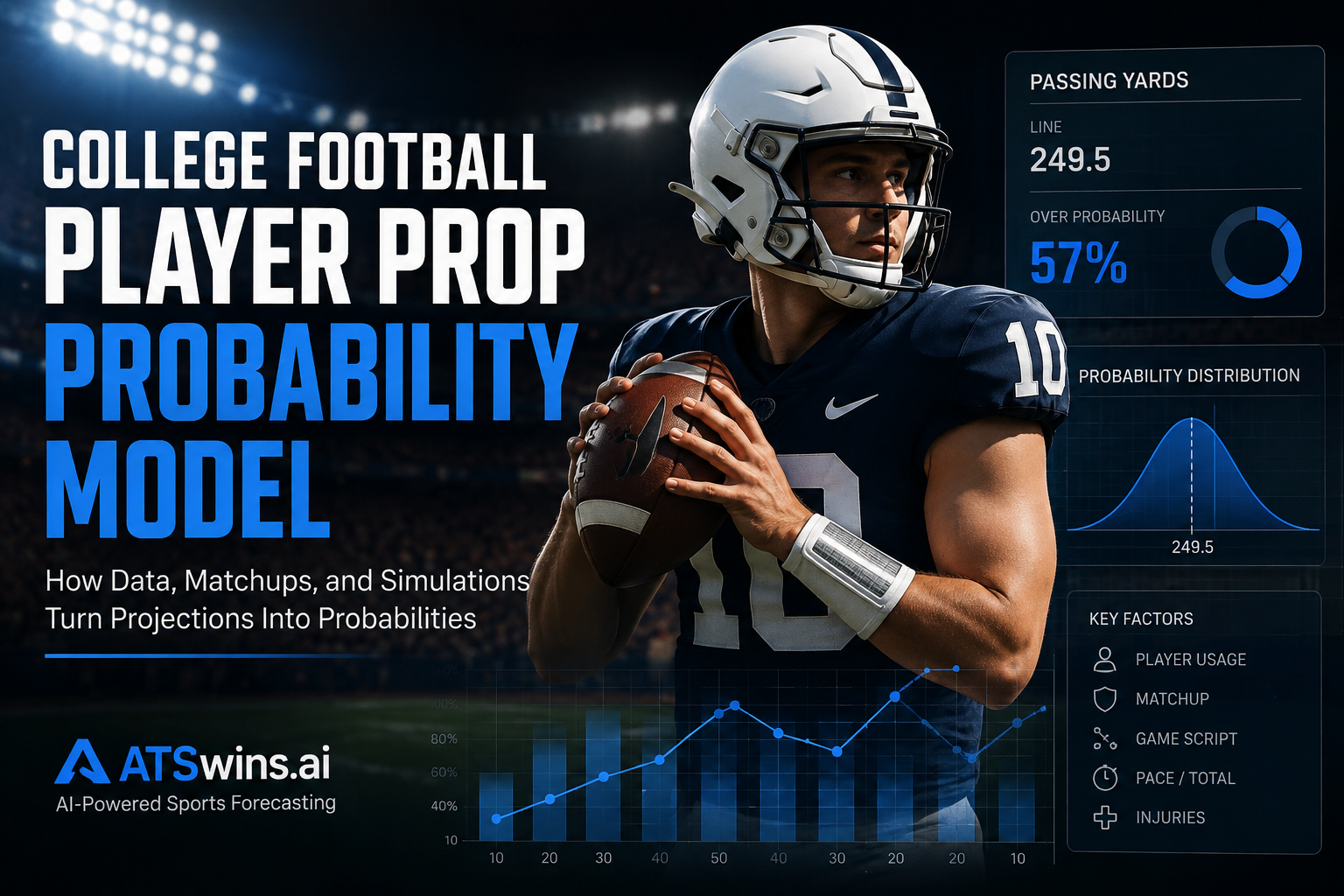
College football player prop probability models estimate how likely a specific player is to finish above or below a betting line. Instead of treating a prop as a simple over-or-under prediction, the model attempts to estimate the full distribution of possible outcomes and then calculate the probability that the player lands on either side of the number.
For example, if a quarterback has a passing-yard prop of 249.5 yards, a useful model does not simply predict 257 yards and call it an over. It estimates the player's expected passing volume, efficiency, matchup, game environment, and uncertainty, then determines how often the simulated outcomes exceed 249.5.
That distinction matters because a prediction and a probability are not the same thing. A player projected for 257 yards could still have only a 55% chance of going over a 249.5-yard line.
College football player props commonly include passing yards, passing attempts, passing touchdowns, rushing yards, rushing attempts, receptions, receiving yards, and anytime touchdown markets.
Table of Contents
- What a College Football Player Prop Probability Model Does
- The Data Behind a Player Prop Probability Model
- How the Model Turns Player Data Into Probability
- Why Game Environment Matters
- A Practical Passing-Yards Example
- Probability Versus Sportsbook Odds
- How Injuries and Role Changes Affect the Model
- Common Problems With College Football Prop Models
- How ATSwins Approaches Probability-Based Analysis
- Why Calibration Matters More Than Confidence
- Final Takeaway
- Frequently Asked Questions
What a College Football Player Prop Probability Model Does
The basic objective is straightforward: estimate the probability of a player reaching a specific statistical threshold.
Suppose a running back has a rushing-yard line of 84.5 yards. A probability model might estimate that he has a 58% chance of finishing above the line and a 42% chance of finishing below it.
That output is more useful than simply saying the running back is projected for 88 rushing yards.
The 88-yard projection represents an expected outcome. The 58% figure describes the uncertainty surrounding that expectation.
That uncertainty is especially important in college football because player usage can vary significantly from game to game. A running back may receive 22 carries in a competitive game but only 11 attempts if his team builds a large lead. A receiver may have a large target share one week and disappear the next because of coverage, game plan, or changes in personnel.
A good probability model therefore needs to account for more than historical averages.
The goal is not to predict exactly what will happen. The goal is to estimate the distribution of realistic outcomes well enough to determine how frequently a particular prop line would be exceeded.
The Data Behind a Player Prop Probability Model
A college football player prop model begins with clean historical data.
For a quarterback, useful inputs might include passing attempts, completion rate, yards per attempt, touchdown rate, interception rate, pressure rate, rushing involvement, opponent pass defense, projected game script, and expected possessions.
For a running back, the model might consider rushing attempts, yards per carry, explosive-run rate, red-zone opportunities, goal-line usage, receiving involvement, offensive-line performance, opponent run defense, and expected score differential.
Receivers require another layer of usage analysis. Targets, target share, route participation, average depth of target, receptions per target, yards per route, red-zone targets, and opponent coverage tendencies can all influence the projection.
Raw season averages should rarely be used by themselves.
A player averaging 92 rushing yards per game against weak defenses does not necessarily have a 92-yard expectation against an elite run defense. Similarly, a receiver averaging seven catches per game may have a different outlook if his quarterback is expected to face heavy pressure.
Opponent-adjusted metrics help account for these differences.
Recency also matters, but it needs to be handled carefully. A recent change in playing time may contain useful information, while a single unusually efficient game can create misleading noise.
A strong model usually blends recent performance with larger-sample historical information rather than completely replacing one with the other.
How the Model Turns Player Data Into Probability
There are several ways to build a college football player prop probability model.
A relatively simple approach begins with a statistical distribution around the player's expected output.
For a rushing-yard prop, the model could estimate expected carries and expected yards per carry, then simulate the resulting rushing totals. For receptions, it could model targets first and then estimate the probability of each target becoming a catch.
More sophisticated systems can use gradient-boosting models such as XGBoost or LightGBM to estimate expected production, followed by a separate distribution or simulation layer.
The important point is that the model should not stop at a single projected number.
Imagine a model projects a receiver for 63 receiving yards. That projection could come from very different distributions.
One player might have outcomes concentrated around 63 yards, with most simulations landing between 45 and 80 yards.
Another player might have a much wider distribution, with frequent outcomes around 20 yards but occasional games above 120.
Both players could have the same 63-yard mean, but their probabilities of clearing a 59.5-yard prop would be very different.
That is why probability modeling requires an understanding of variance.
Monte Carlo simulation is one practical way to represent that uncertainty. A model can simulate a large number of possible game scenarios using its assumptions about volume, efficiency, pace, opponent strength, and game script. The percentage of simulations that exceed the prop line becomes the estimated over probability.
Computer simulation is already used by some publicly available college football prop systems, illustrating the broader direction of modern player-prop analysis.
Why Game Environment Matters
A player does not produce statistics in isolation.
Game environment can change the number of opportunities available to almost every player on the field.
A quarterback facing an opponent that is expected to score efficiently may have to throw more often. That can increase passing attempts and potentially passing yards.
The same game could hurt a running back's rushing volume if his team is expected to play from behind.
A favorite in a projected blowout presents the opposite problem. The offense could score efficiently while reducing the starter's workload during the second half.
Possessions matter too. A faster game creates more opportunities, while a slower game can reduce total plays.
The model should therefore incorporate team pace, expected scoring, spread, total, opponent tendencies, and projected game script when those variables provide meaningful predictive information.
Weather can matter as well, particularly for outdoor games. Wind can affect passing efficiency and kicking, while heavy precipitation can alter play selection and field conditions. The impact should be quantified rather than automatically treated as a reason to bet an under.
The same principle applies to home-field advantage, travel, rest, and altitude. None should be treated as magic variables. Their usefulness depends on whether historical data demonstrates a repeatable relationship with the statistic being modeled.
A Practical Passing-Yards Example
Consider a hypothetical quarterback with a passing-yard prop of 249.5.
A model might project:
Expected attempts: 35.2
Expected completion rate: 64%
Expected yards per attempt: 7.4
Expected passing yards: approximately 260
At first glance, a 260-yard projection looks like a straightforward over.
But now suppose the model runs 25,000 simulated game outcomes. The results might show that the quarterback clears 249.5 yards in 57% of simulations.
That means the model's estimated probability of the over is 57%.
Now consider a different quarterback with the same 260-yard projection. If his distribution is much narrower, perhaps 64% of simulations could exceed 249.5.
The two quarterbacks have identical mean projections but very different probabilities.
This illustrates why player-prop modeling should focus on distributions rather than projections alone.
It also explains why simply comparing a player's season average with a sportsbook line is often inadequate. A season average does not tell you how the player's usage has changed, how difficult the matchup is, or how wide the expected outcome distribution is.
Probability Versus Sportsbook Odds
Once a model produces a probability, the next question is whether that probability differs meaningfully from the market price.
Suppose a sportsbook lists a prop at -115.
Ignoring the bookmaker's margin, the implied probability of -115 is approximately 53.5%.
If a model estimates the true probability at 58%, there is a difference between the market's implied probability and the model's estimate.
That difference is potentially useful, but it should not automatically be treated as a guaranteed advantage.
Model error matters.
If the model is poorly calibrated and routinely overstates probabilities, a reported 58% probability might actually behave more like a 53% probability.
This is why fair probability and available betting price should be treated as separate concepts.
A model can estimate that an outcome has a 60% probability while the available price still may not provide enough value after accounting for the vig.
The goal is not simply to find the props most likely to hit. A -300 prop might have a much higher hit probability than a +200 prop, but the price determines whether that probability creates a worthwhile expected-value situation.
How Injuries and Role Changes Affect the Model
College football player props become especially difficult when player roles change.
An injury to a starting running back can increase the workload of a backup. But the backup should not automatically inherit 100% of the starter's previous carries.
The coaching staff may use a committee approach. Another running back could absorb some snaps. The team could also change its offensive strategy.
The same issue appears with receivers.
If a starting wide receiver is unavailable, the next player on the depth chart might receive additional routes and targets. But those opportunities are distributed across the entire offense.
A probability model should therefore treat injuries as changes to expected usage rather than simple one-for-one statistical substitutions.
Quarterback changes can be even more complicated.
A backup quarterback may have different passing efficiency, scrambling tendencies, and decision-making characteristics. That can change the projections for every skill-position player on the offense.
The model should update the entire offensive environment when a major personnel change occurs.
Common Problems With College Football Prop Models
One of the biggest problems is small sample size.
College football players often have limited career samples, and some players experience dramatic role changes between seasons. A model that heavily weights a player's last four games can become unstable.
Data leakage is another major problem.
A model should only use information that would have been available at the time the prediction was made. Using final-season statistics to recreate an earlier-season prediction produces artificially strong backtests.
Time-aware validation is therefore essential.
Historical games should be separated chronologically so that future information does not leak into earlier predictions.
Another problem is ignoring market movement.
A prop may open at 65.5 yards and move to 71.5 after significant information reaches the market. A model's probability needs to be evaluated against the actual price and line available at the intended betting time.
There is also the problem of overconfidence.
A model producing an 80% probability does not mean the event is certain. Even a properly calibrated 80% probability means the outcome should fail roughly 20% of the time over a sufficiently large sample.
Random variance never disappears.
How ATSwins Approaches Probability-Based Analysis
ATSwins is built around the idea that sports forecasting should be treated as a probability problem rather than a collection of confident predictions.
For college football player props, that means separating the player's projected performance from the probability of reaching a specific market line.
A useful analytical workflow starts with player usage and historical production, then incorporates opponent quality, expected game environment, role, injuries, and other relevant information. The resulting projection can then be translated into a probability distribution and compared with the market.
That distinction fits naturally with ATSwins' broader focus on statistical modeling, player projections, probability analysis, fair-line estimates, simulations, and market evaluation.
The objective is not to pretend that a model knows exactly what will happen on Saturday.
It is to quantify what the available data suggests and make the uncertainty visible.
For example, a model might project a receiver for 71 yards but estimate only a 54% probability of exceeding a 69.5-yard line. That is a very different conclusion from simply labeling the player an "over" based on the 71-yard projection.
The probability provides the context that the projection alone cannot.
Why Calibration Matters More Than Confidence
Calibration is one of the most overlooked parts of sports probability modeling.
Suppose a model labels 1,000 outcomes as having a 70% probability of occurring. If the model is well calibrated, approximately 700 of those outcomes should actually occur.
If only 590 happen, the model is systematically overconfident.
If 790 happen, it is systematically underconfident.
A model can therefore have reasonable predictive accuracy while still producing poorly calibrated probabilities.
For betting-market analysis, that distinction matters because probability is directly connected to price.
Calibration methods such as Platt scaling and isotonic regression can be applied after a predictive model is trained. Historical predictions can then be compared with actual outcomes to determine whether the probabilities behave as expected.
Calibration should also be evaluated across different prop types.
A model might be well calibrated for passing yards but less reliable for anytime touchdowns. Touchdowns are relatively low-frequency events and often have more variance, making them particularly difficult to estimate.
The model should not assume that one probability framework works equally well across every market.
Building a Better College Football Player Prop Probability Model
A useful system does not need to be unnecessarily complicated.
The most important foundation is reliable, time-stamped data.
From there, the model should establish reasonable player baselines and adjust them for current role, opponent, expected volume, efficiency, and game context.
The next step is converting those projections into distributions rather than stopping at point estimates.
Simulation can then estimate the probability of clearing different prop lines.
Finally, the probabilities should be calibrated and evaluated through historical backtesting.
The evaluation should measure more than whether individual props won or lost. Brier score, log loss, calibration curves, closing-line value, expected value, and performance across different market conditions can provide a more complete picture of model quality.
That process also makes it easier to identify where the model is weak.
A model may perform well on rushing-yard props but struggle with touchdown markets. It may be strong on established starters but weaker when freshmen or backups suddenly receive major workloads.
Those weaknesses should be measured rather than hidden behind a single overall accuracy number.
Final Takeaway
A college football player prop probability model is more than a system that predicts how many yards a player will gain.
The useful output is a probability distribution that accounts for player usage, opponent quality, game environment, injuries, role changes, expected volume, efficiency, and uncertainty.
A projection tells you what the model expects.
A probability tells you how often the model expects a specific outcome to occur.
The difference is critical when evaluating a betting line.
A strong model also recognizes its own limitations. College football contains substantial player turnover, changing roles, uneven sample sizes, coaching adjustments, injuries, and random variance. No probability model eliminates those factors.
ATSwins approaches sports analytics from that probability-first perspective, using projections and market evaluation as tools for disciplined decision-making rather than guarantees about future results.
The better question is not simply, "Will this player go over?"
It is, "Given everything known before the game, how likely is the player to clear this exact number, and how does that probability compare with the available price?"
That is the foundation of serious player-prop modeling.