

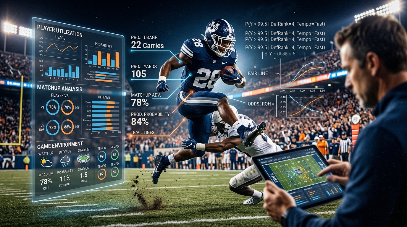
College football player props are harder to project than they first appear. A quarterback's passing yards depend on expected plays, pass rate, pressure, game script, and efficiency. A running back's rushing total depends on workload, offensive line performance, opponent strength, and whether the game stays competitive. A receiver's projection depends on routes, targets, quarterback tendencies, coverage, and team passing volume.
That is why a college football player prop prediction model should not simply average a player's last few games. A stronger model estimates expected opportunity first, adjusts that opportunity for matchup and game conditions, and then converts the result into a probability distribution. The goal is not to claim exactly what a player will produce. It is to estimate the range of outcomes and determine how likely different results are.
This approach is especially useful in college football because rosters and roles change quickly. NCAA statistics provide individual categories such as passing yards, rushing yards, receiving yards, receptions, and touchdowns, while more detailed college football datasets can provide play-by-play, player usage, weather, and advanced metrics.
Table of Contents
What a College Football Player Prop Model Projects
The Data Inputs Behind Player Projections
Why Usage and Matchup Matter
Turning a Projection Into Probability
A Simple Player Prop Modeling Example
How to Validate the Model
How ATSwins Fits Into the Process
Where Player Prop Models Can Fail
Building Better College Football Projections
Frequently Asked Questions
What a College Football Player Prop Model Projects
A player prop model starts with a specific statistical target. Common examples include passing yards, passing attempts, rushing yards, rushing attempts, receptions, receiving yards, and touchdowns.
The target matters because different statistics behave differently. Passing yards have a relationship with attempts and yards per attempt. Rushing yards are strongly tied to carries and yards per carry. Receptions depend on routes, targets, catch rate, and offensive passing volume. Touchdowns are much more volatile because relatively few scoring events determine the result.
The model should therefore not treat every prop as the same prediction problem.
For example, projecting a quarterback for 275 passing yards can be broken into expected pass attempts multiplied by expected yards per attempt. A receiver's receiving-yard projection might begin with expected targets, estimated catch rate, and expected yards per reception.
That decomposition gives the model something useful to learn. Instead of asking only how many yards a player will get, it asks how much opportunity the player is likely to receive and how productive that opportunity could be.
That distinction becomes critical when a player's role changes.
The Data Inputs Behind Player Projections
A serious NCAAF player projection model needs more than season averages.
The NCAA's official football statistics include individual categories such as passing yards, passing touchdowns, rushing yards, rushing touchdowns, receptions, receiving yards, and yards per reception. Those statistics provide a useful starting point, but stronger models can combine them with more granular information.
The College Football Data API provides access to game, play-by-play, player, usage, weather, advanced statistics, predicted points added, and adjusted player metrics. That type of information can be used to construct features for a college football player prop prediction model.
Player history provides recent production, workload, efficiency, and consistency. Team information adds offensive pace, passing rate, rushing tendencies, scoring environment, and expected play volume. Opponent information provides defensive efficiency and matchup characteristics. Game context adds home or away status, expected competitiveness, weather, and potential game script.
Roster information is particularly important in college football. A player may have a limited historical sample because he transferred, became a starter, changed positions, or moved into a larger role.
A model that blindly treats last season's statistics as equally predictive can become stale quickly.
This is where weighted historical data becomes useful. Recent games can receive greater weight while older results still provide a stabilizing baseline.
Why Usage and Matchup Matter More Than Raw Averages
A raw average can hide the most important part of a player prop: opportunity.
Suppose a running back averaged 82 rushing yards over his last four games. That sounds useful, but it does not tell us whether the player received 14 carries, 22 carries, or 28 carries per game.
If the player's workload increased from 14 carries to 23 carries, the model should recognize that the underlying opportunity changed.
The same principle applies to receivers whose route participation or targets increase after another player leaves the lineup.
A useful model can estimate expected workload first and efficiency second.
For a simplified rushing model:
Expected rushing yards = expected carries × expected yards per carry
The two components can then be adjusted independently.
Expected carries may depend on recent snap share, team rushing rate, score differential, coaching tendencies, and opponent matchup. Expected yards per carry can incorporate the player's historical efficiency, opponent rushing defense, offensive line performance, and game environment.
Passing and receiving models can use a similar structure.
This also explains why matchup data should not simply be represented as "defense ranks 20th against the run."
Rankings compress a lot of information into one number. A model can instead examine efficiency allowed, explosive plays, opponent-adjusted performance, pace, and the type of workload the defense tends to concede.
The goal is not to find one magic statistic. It is to combine several imperfect signals without allowing correlated features to overwhelm the model.
Turning a Projection Into Probability
One of the biggest differences between a basic projection and a useful player prop model is the treatment of uncertainty.
Suppose a model projects a running back for 94 rushing yards. That does not mean the player is expected to land exactly at 94.
The actual distribution could contain outcomes from 35 yards to 160 yards, with different probabilities across that range.
A model can estimate this distribution using regression techniques, count models, simulation, or other distributional approaches depending on the statistic.
Once the distribution exists, a prop line can be evaluated.
Imagine a hypothetical market line of 84.5 rushing yards and a model projection of 94 yards. The difference is 9.5 yards, but that difference alone does not tell us whether the over is attractive.
The model needs to estimate:
P(rushing yards > 84.5)
If that probability is 58%, the model is saying the player exceeds the number more often than a 50/50 outcome.
If the probability is only 51%, the same 94-yard projection might not justify much interest because the distribution could be wide.
This is why probability is more informative than a point projection by itself.
A fair price can then be derived from the model probability. For example, a 58% probability corresponds to decimal fair odds of approximately 1.72 before accounting for additional market considerations.
The market price and model probability should remain separate concepts. A model does not create an edge merely because its projection is higher than a prop line.
A Simple Player Prop Modeling Example
Consider a hypothetical college running back with an upcoming rushing-yards prop of 79.5.
The model estimates his workload at 19 carries. His baseline efficiency is 4.8 yards per carry, but the opponent adjustment lowers expected efficiency to 4.5.
The initial projection becomes:
19 carries × 4.5 yards = 85.5 rushing yards
That 85.5 number is only the center of the forecast.
The model then introduces uncertainty around carries and efficiency. Perhaps a negative game script reduces the workload, while a competitive game creates more opportunities. Weather may also affect play selection and efficiency.
After simulation, the model might estimate that the player clears 79.5 yards in 56% of scenarios.
That result is more useful than simply saying "projection: 85.5."
Now suppose the market moves from 79.5 to 86.5. The underlying player projection has not changed, but the probability of clearing the line has.
The model should therefore be evaluated against the new number.
This illustrates an important principle: the value of a player prop depends on both the player's projected distribution and the price being offered.
A projection is not permanently attached to a betting line.
How to Validate a College Football Player Prop Model
A model that performs well on historical data can still fail badly in live use if the testing process is flawed.
The first issue is time leakage.
A model predicting Week 6 should not have access to information that became available after Week 6. Training and validation should respect the chronology of the season.
Walk-forward validation is a practical approach. The model can train on earlier games, predict a later group of games, record the results, and then move forward through the schedule.
This structure better represents how the model will operate during a real season.
Evaluation should also go beyond simple hit rate.
For probability forecasts, Brier score and log loss are useful because they evaluate the quality of predicted probabilities. Calibration is equally important.
If a model labels outcomes as 60% likely, those events should occur at roughly the expected rate across a sufficiently large sample.
Regression accuracy can also be evaluated with metrics such as mean absolute error.
But even a low average error does not guarantee useful prop probabilities. A model could consistently project close to the mean while failing to understand extreme outcomes.
That matters because player props are often decided by tail outcomes.
Validation should also separate different situations. Early-season games, conference play, rivalry games, bowl games, major role changes, and injury replacements may behave differently.
A model should be tested against simple baselines as well. If a complex machine-learning system cannot consistently improve on a basic usage-plus-efficiency model, complexity may be adding noise rather than information.
How ATSwins Fits Into the Process
ATSwins approaches sports forecasting around probabilities, projections, market evaluation, and data-driven analysis rather than treating a prediction as a certainty.
That same philosophy makes sense for player props.
A player projection should be viewed alongside the surrounding game environment. If a quarterback is projected for high passing volume because his team is expected to trail, that same game script may increase opportunities for his leading receiver while reducing rushing attempts for the running back.
Those relationships matter because player props are not independent islands.
A useful forecasting workflow can therefore connect team-level projections with player-level usage.
Team pace influences total plays. Expected team points influence touchdown opportunities. Expected game script influences passing and rushing volume. Injuries alter depth charts and redistribute opportunity.
This creates a more complete picture than simply taking a player's season average and comparing it with a prop line.
For ATSwins, that broader analytical framework fits naturally with college football forecasting because player outcomes are connected to team performance, opponent strength, situational factors, and market expectations.
Where Player Prop Models Can Fail
No college football player prop prediction model eliminates uncertainty.
Injuries are an obvious problem. A player can be technically active but receive fewer snaps because of a limitation that is difficult to quantify before kickoff. Depth-chart changes can also happen quickly.
Small samples create another issue.
A backup receiver might have three excellent games after becoming a starter, but three games are not necessarily enough to establish his long-term efficiency.
Coaching decisions are difficult to forecast as well. A team may unexpectedly abandon its normal run-pass balance because of opponent tendencies, weather, or an early-game result.
College football also contains substantial roster turnover. Transfers, freshmen, coaching changes, and evolving roles can make historical data less transferable than it appears.
There is also correlation between player props.
A quarterback over on passing yards and his top receiver over on receiving yards may be linked by the same underlying game environment. Treating those positions as completely independent can underestimate portfolio risk.
Finally, model uncertainty itself needs to be measured.
If two reasonable models produce projections of 82 and 96 yards, presenting a single number such as 89 without showing the uncertainty can create false precision.
A good forecasting system should know when its confidence is low.
Building Better College Football Projections
A reliable college football player prop prediction model starts with the player's expected opportunity and then layers in efficiency, opponent strength, game environment, injuries, roster changes, and uncertainty.
The strongest approach is not necessarily the most complicated one.
A transparent model with good data, sensible features, time-aware validation, and calibrated probabilities can be more useful than an overly complex system trained on noisy historical relationships.
The key distinction is between saying a player is projected for 85 yards and estimating the probability that he clears a specific market number.
The first is a projection.
The second is a probability problem tied to a price.
That distinction fits the broader ATSwins philosophy of using sports data to understand probabilities and market context rather than presenting forecasts as guarantees.
For readers interested in college football player projections, ATSwins provides a useful framework for thinking about player props through data, simulations, probabilities, and broader game context.
Frequently Asked Questions
What is a college football player prop prediction model?
A college football player prop prediction model is a statistical system that estimates an individual player's expected performance for a specific category, such as passing yards, rushing yards, receptions, receiving yards, or touchdowns.
More advanced models estimate a probability distribution rather than only producing one projected number.
That allows the model to estimate the probability that a player goes over or under a specific market line.
What data should a CFB player prop model use?
A useful model can combine player statistics, snap or usage data, team pace, play volume, opponent defensive performance, game script, injuries, weather, home-field context, and roster information.
The most important part is not simply collecting as many variables as possible. The variables need to have a logical relationship with the statistic being projected and should be tested carefully to avoid overfitting.
Are college football player projections the same as betting predictions?
No.
A projection estimates a player's expected statistical outcome. A betting prediction requires another step because the projection must be compared with a specific market line and price.
An 85-yard projection means something different against a 70.5-yard line than it does against a 94.5-yard line.
Probability and price therefore matter alongside the projection.
How do you account for injuries and role changes?
The model should update player usage expectations when relevant information changes.
A starter's absence can increase another player's expected snaps, carries, targets, or routes.
The challenge is avoiding overreaction to uncertain information. Historical data can provide a baseline while current depth-chart and availability information shifts the forecast.
Can an AI model accurately predict college football player props?
AI and machine-learning methods can process large amounts of player, team, opponent, and contextual data, but they cannot remove randomness from football.
The quality of the underlying data, feature design, validation process, calibration, and timing of information all affect the result.
A well-calibrated probability forecast is generally more informative than claiming that a model knows exactly what will happen.